有时在研究过程中,需要用到理论正演数据的初至,如果手动拾取的话…想想都头大,本文提供一种计算理论正演地震数据初至的方法。
1. 数据准备
首先,准备一下数据,去SEG Open data下载一个2D Walkaway VSP的正演数据。
1 | import numpy as np |
看下数据长啥样:(其中read_segy可以参考这篇笔记:Python读写segy数据)
1 | model_vsp = read_segy.read_segy(data_dir='F:/data/SEAM_I_Walkaway_VSP/SEAM_Well1VSP_Shots23900.sgy',shotnum=0) |
2. 计算初至的函数
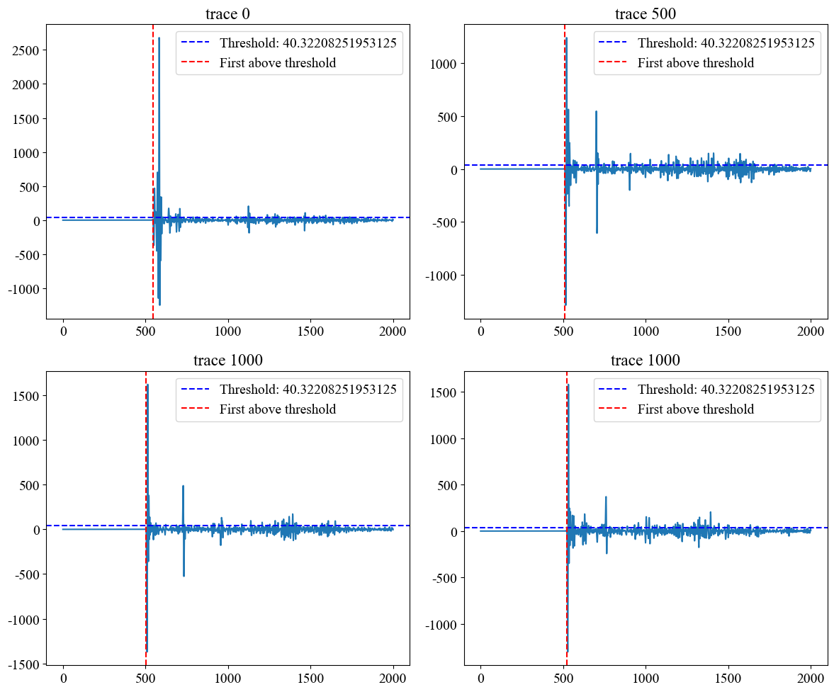
定义计算初至的函数,思路为找到超过该道最大振幅值*相对阈值的第一个点。
(一开始是计划找到不为0的第一个点,但是会受到一些随机噪声的影响,故放弃)
1 | def calculate_fb(seismic_data, threshold=0.01): |
3. 计算单炮的初至,检查结果
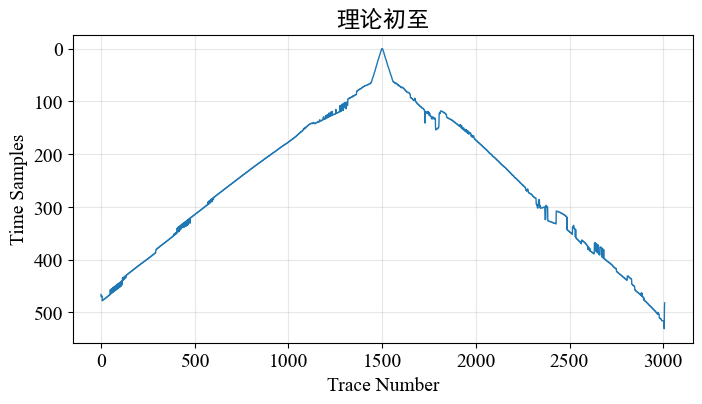
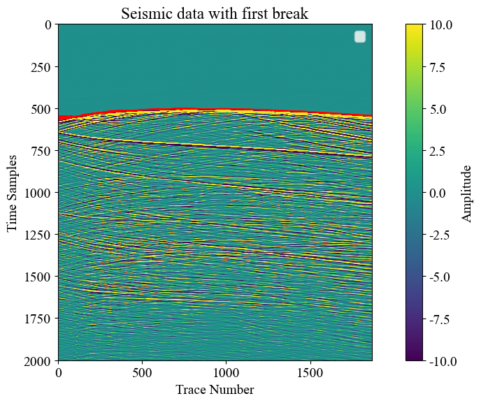
计算该数据第0炮的初至,并画图看看:
1 | fb = calculate_fb(model_vsp[0],threshold=0.01) |
检查一下单道的拾取位置是否正确
1 | # 检查其中4道吧 |
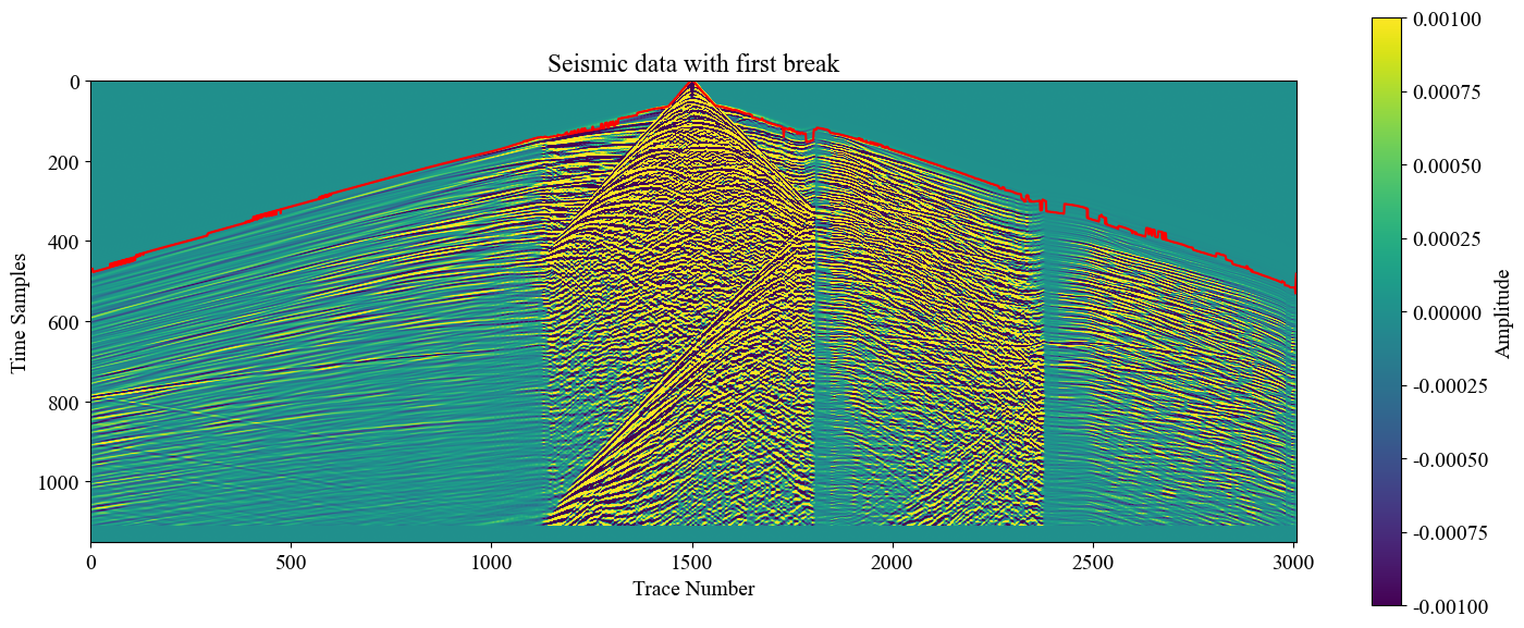
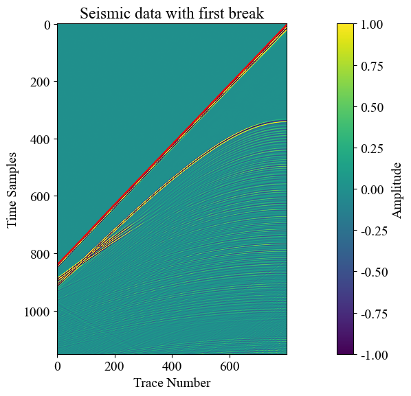
绘制地震单炮和计算出的初至,叠合显示,检查结果是否正确:
1 | plt.figure(figsize=(10, 6)) |
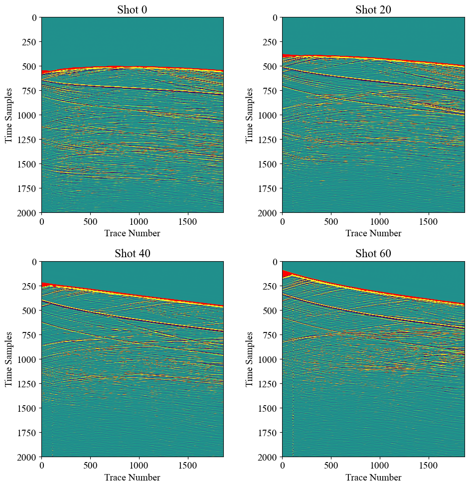
4. 计算所有炮的初至
1 | shots, times, traces = model_vsp.shape |
检查一下结果:
1 | fig, axes = plt.subplots(2, 2, figsize=(10, 10)) |
The end
当然,本文只提供一种初至的近似解,如果数据质量好的话,初至当然比较完美,如果数据质量差的话,肯定也会有一些瑕疵。
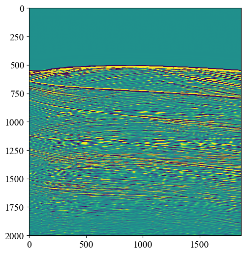
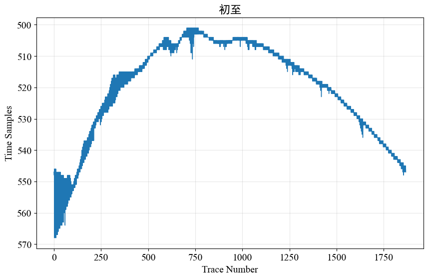
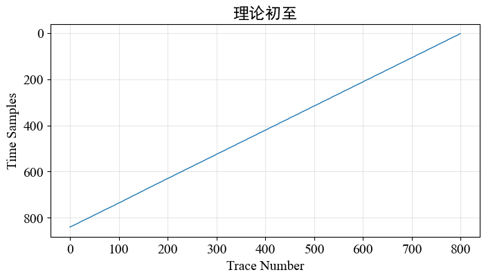
例如下面两组数据:数据来源:第一个数据model_ani, 第二个数据model_7m
1 | fb = calculate_fb(model_ani[0],threshold=0.01) # model_7m[0] |
model_ani 初至计算结果:
model_7m 初至计算结果: