1
2
3
4
5
6
7
8
9
10
11
12
13
14
15
16
17
18
19
20
21
22
23
24
25
26
27
28
29
30
31
32
33
34
35
36
37
38
39
40
41
42
43
44
45
46
47
48
49
50
51
52
53
54
55
56
57
58
59
60
61
62
63
64
65
66
67
68
69
70
71
72
73
74
75
76
77
78
79
80
81
82
83
84
85
| function ShowMT1DForward_withorwithoutBakken(varargin)
f = logspace(-3,3,21)';
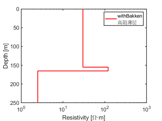
rho_withBakken = [30;120;2.5];
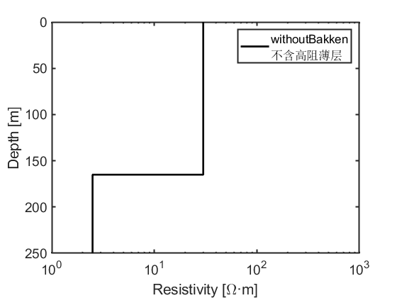
rho_withoutBakken = [30;30;2.5];
h = [155;10];
[x,y] = Getxy(rho_withBakken,h,85);
figure,
semilogx(x,y,'-r','LineWidth',2.0);
axis([10^0,10^3,-inf,inf]);
set(gca,'YDir','rev','LineWidth',1.5,'FontSize',14);
xlabel('Resistivity [\Omega·m]');
ylabel('Depth [m]');
legend(['withBakken',newline,'高阻薄层']);
[x1,y1] = Getxy(rho_withoutBakken,h,85);
figure,
semilogx(x1,y1,'-k','LineWidth',2.0);
axis([10^0,10^3,-inf,inf]);
set(gca,'YDir','rev','LineWidth',1.5,'FontSize',14);
xlabel('Resistivity [\Omega·m]');
ylabel('Depth [m]');
legend(['withoutBakken',newline,'不含高阻薄层']);
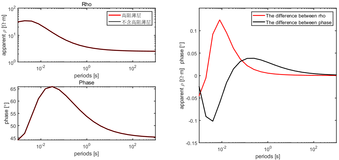
[apparentRho_1,Phase_1]=MT1DForward(rho_withBakken,h,f);
[apparentRho_2,Phase_2]=MT1DForward(rho_withoutBakken,h,f);
figure,
subplot(2,2,1)
plot(1./f,apparentRho_1,'-r','LineWidth',2.5)
hold on;
plot(1./f,apparentRho_2,'-k','LineWidth',1.5)
set(gca,'Yscale','log','Xscale','log','LineWidth',1.5,'FontSize',12)
xlabel('periods [s]');
ylabel('apparent \rho [\Omega·m]')
title('Rho');
axis([10^-3,10^3,10^0,10^2]);
legend('高阻薄层','不含高阻薄层','FontSize',12);
subplot(2,2,3)
plot(1./f,Phase_1,'-r','LineWidth',2.5)
hold on;
plot(1./f,Phase_2,'-k','LineWidth',1.5)
set(gca,'Xscale','log','LineWidth',1.5,'FontSize',12)
xlabel('periods [s]');
ylabel('phase [\circ]');
title('Phase');
axis([10^-3,10^3,-inf,inf]);
subplot(2,2,[2,4])
plot(1./f,apparentRho_1-apparentRho_2,'-r','LineWidth',2.0)
hold on;
plot(1./f,Phase_1-Phase_2,'-k','LineWidth',2.0)
set(gca,'Xscale','log','LineWidth',1.5,'FontSize',12)
axis([10^-3,10^3,-0.15,0.15]);
xlabel('periods [s]');
ylabel('apparent \rho [\Omega·m] phase [\circ]');
legend('The difference between rho','The difference between phase','FontSize',12);
set(gcf,'unit','normalized','position',[0.2,0.2,0.7,0.5]);
end
function [x,y] = Getxy(rho, h, deep)
Depth(1) = 0;
y(1) = Depth(1);
if length(rho)>=2
for j=2:length(rho)
Depth(j) = Depth(j-1)+h(j-1);
y(2*j-2) = Depth(j);
y(2*j-1) = Depth(j);
end
y(2*j) = y(2*j-1) + deep;
else
y(2) = 1000;
end
for j=1:length(rho)
x(2*j-1)=rho(j);
x(2*j)=rho(j);
end
end
|