1
2
3
4
5
6
7
8
9
10
11
12
13
14
15
16
17
18
19
20
21
22
23
24
25
26
27
28
29
30
31
32
33
34
35
36
37
38
39
40
41
42
43
44
45
46
47
48
49
50
51
52
53
54
55
56
57
58
59
60
61
62
63
64
65
66
67
68
69
70
71
72
73
74
75
76
77
78
79
80
81
82
83
84
85
86
87
88
89
90
91
92
93
94
95
96
97
98
99
100
101
102
103
104
105
106
107
108
109
110
111
112
113
114
115
116
117
118
119
120
121
122
123
124
|
clear;
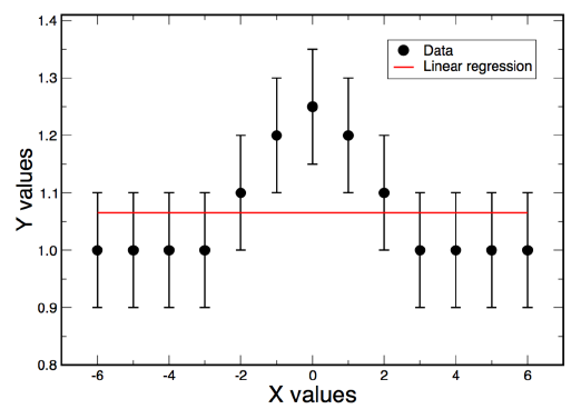
x = -6:1:6;
y = [1,1,1,1,1.1,1.2,1.25,1.2,1.1,1,1,1,1];
scatter(x,y,'filled','k','LineWidth',2);
axis([-7 7 0.8 1.4]);
x1= -6:0.1:6;
hold on;
[p1,s1] = polyfit(x,y,1);
[y1,s1] = polyval(p1,x,s1);
plot(x1, polyval(p1, x1),'r','LineWidth',2);
hold on;
[p2,s2] = polyfit(x,y,2);
[y2,s2] = polyval(p2,x,s2);
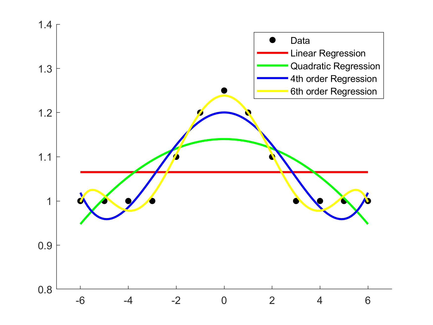
plot(x1, polyval(p2, x1),'g','LineWidth',2);
hold on;
[p3,s3] = polyfit(x,y,4);
[y3,s3] = polyval(p3,x,s3);
plot(x1, polyval(p3, x1),'blue','LineWidth',2);
hold on;
[p4,s4] = polyfit(x,y,6);
[y4,s4] = polyval(p4,x,s4);
plot(x1, polyval(p4, x1),'y','LineWidth',2);
legend('Data','Linear Regression','Quadratic Regression','4th order Regression','6th order Regression');
ans1 = 1.065;
ans2 = -0.0053447* x.^2 + 1.1402;
ans3 = 0.00041821* x.^4 - 0.020101* x.^2 + 1.2004;
ans4 = -2.924e-05* x.^6 + 0.0019998* x.^4 - 0.040793* x.^2 + 1.2387;
n = numel(x);
Misfit1 = sum(power(y-ans1,2))*100;
RMS1_ = sqrt(Misfit1/(n-1));
Misfit2 = sum(power(y-ans2,2)*100);
RMS2_ = sqrt(Misfit2/(n-1));
Misfit3 = sum(power(y-ans3,2))*100;
RMS3_ = sqrt(Misfit3/(n-1));
Misfit4 = sum(power(y-ans4,2))*100;
RMS4_ = sqrt(Misfit4/(n-1));
n = numel(x);
dataMisfit1 = sum(power(y-y1,2));
nRMS1 = sqrt(dataMisfit1/(n-1));
dataMisfit2 = sum(power(y-y2,2)./power(s2,2));
nRMS2 = sqrt(dataMisfit2/(n-1));
dataMisfit3 = sum(power(y-y3,2)./power(s3,2));
nRMS3 = sqrt(dataMisfit3/(n-1));
dataMisfit4 = sum(power(y-y4,2)./power(s4,2));
nRMS4 = sqrt(dataMisfit4/(n-1));
e1=y1 - y;
e1_=mean(e1);
for ie=2:length(e1)
dw_tem1(ie-1)=(e1(ie)-e1(ie-1))^2;
end
for ie=1:length(e1)
dw_tem2(ie)=(e1(ie)-e1_)^2;
end
dw_1=sum(dw_tem1)/sum(dw_tem2);
e2=y2 - y;
e2_=mean(e2);
for ie=2:length(e2)
dw_tem1(ie-1)=(e2(ie)-e2(ie-1))^2;
end
for ie=1:length(e2)
dw_tem2(ie)=(e2(ie)-e2_)^2;
end
dw_2=sum(dw_tem1)/sum(dw_tem2);
e3=y3 - y;
e3_=mean(e3);
for ie=2:length(e3)
dw_tem1(ie-1)=(e3(ie)-e3(ie-1))^2;
end
for ie=1:length(e3)
dw_tem2(ie)=(e3(ie)-e3_)^2;
end
dw_3=sum(dw_tem1)/sum(dw_tem2);
e4=y4 - y;
e4_=mean(e4);
for ie=2:length(e4)
dw_tem1(ie-1)=(e4(ie)-e4(ie-1))^2;
end
for ie=1:length(e4)
dw_tem2(ie)=(e4(ie)-e4_)^2;
end
dw_4=sum(dw_tem1)/sum(dw_tem2);
|