1
2
3
4
5
6
7
8
9
10
11
12
13
14
15
16
17
18
19
20
21
22
23
24
25
26
27
28
29
30
31
32
33
34
35
36
37
38
39
40
41
42
43
44
45
46
47
48
49
50
51
52
53
54
55
56
57
58
59
60
61
62
63
64
65
66
67
68
69
70
71
72
73
74
75
76
77
78
79
80
81
82
83
84
85
86
87
88
89
90
91
92
93
94
95
96
97
98
99
100
101
102
103
104
105
106
107
108
109
110
111
112
113
114
115
116
117
118
119
120
121
122
123
124
125
126
127
128
129
130
|
tic
clear all;
clc;
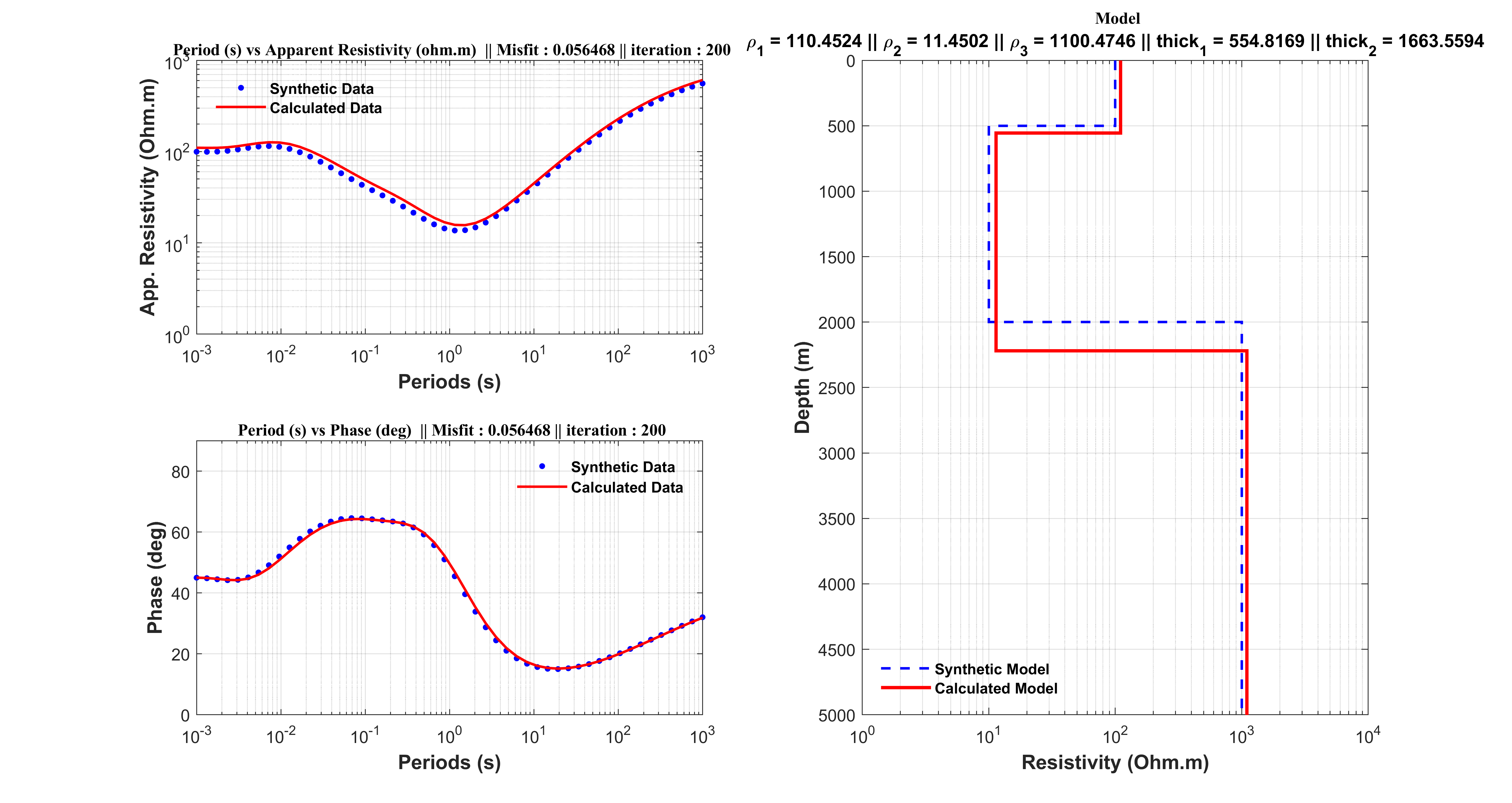
R = [100 10 1000];
thk = [500 1500];
freq = logspace(-3,3,50);
T = 1./freq;
[app_sin, phase_sin] = modelMT(R, thk ,T);
nlayer = 3;
nitr = 200;
LBR = [1 1 1];
UBR = [200 20 2000];
LBT = [1 1];
UBT = [1000 3000];
Temp = 1;
dec = 1;
rho1(1 , :) = LBR + rand*(UBR - LBR);
thick1(1, :) = LBT + rand*(UBT - LBT);
[apparentResistivity1, phase1]=modelMT(rho1(1,:),thick1(1,:),T);
app_mod1(1,:)=apparentResistivity1;
phase_mod1(1,:)=phase1;
[misfit1]=misfitMT(app_sin,phase_sin,app_mod1(1,:),phase_mod1(1,:));
E1=misfit1;
for itr = 1 : nitr
rho_int(1 , :) = LBR + rand*(UBR - LBR);
thick_int(1, :) = LBT + rand*(UBT - LBT);
ui = rand;
yi = sign(ui-0.5)*Temp*((((1 + (1/Temp)))^abs(2*ui-1))-1);
rho2(1 , :) = rho_int + yi*(UBR - LBR);
thick2(1, :) = thick_int + yi*(UBT - LBT);
[apparentResistivity2, phase2]=modelMT(rho2(1,:),thick2(1,:),T);
app_mod2(1,:)=apparentResistivity2;
phase_mod2(1,:)=phase2;
[misfit2]=misfitMT(app_sin,phase_sin,app_mod2(1,:),phase_mod2(1,:));
E2=misfit2;
delta_E = E2 -E1;
if delta_E < 0
rho1 = rho2;
thick1 = thick2;
E1 = E2;
else
P = exp((-delta_E)/Temp);
if P >= rand
rho1 = rho2;
thick1 = thick2;
E1 = E2;
end
end
[apparentResistivity_new, phase_new]=modelMT(rho1(1,:),thick1(1,:),T);
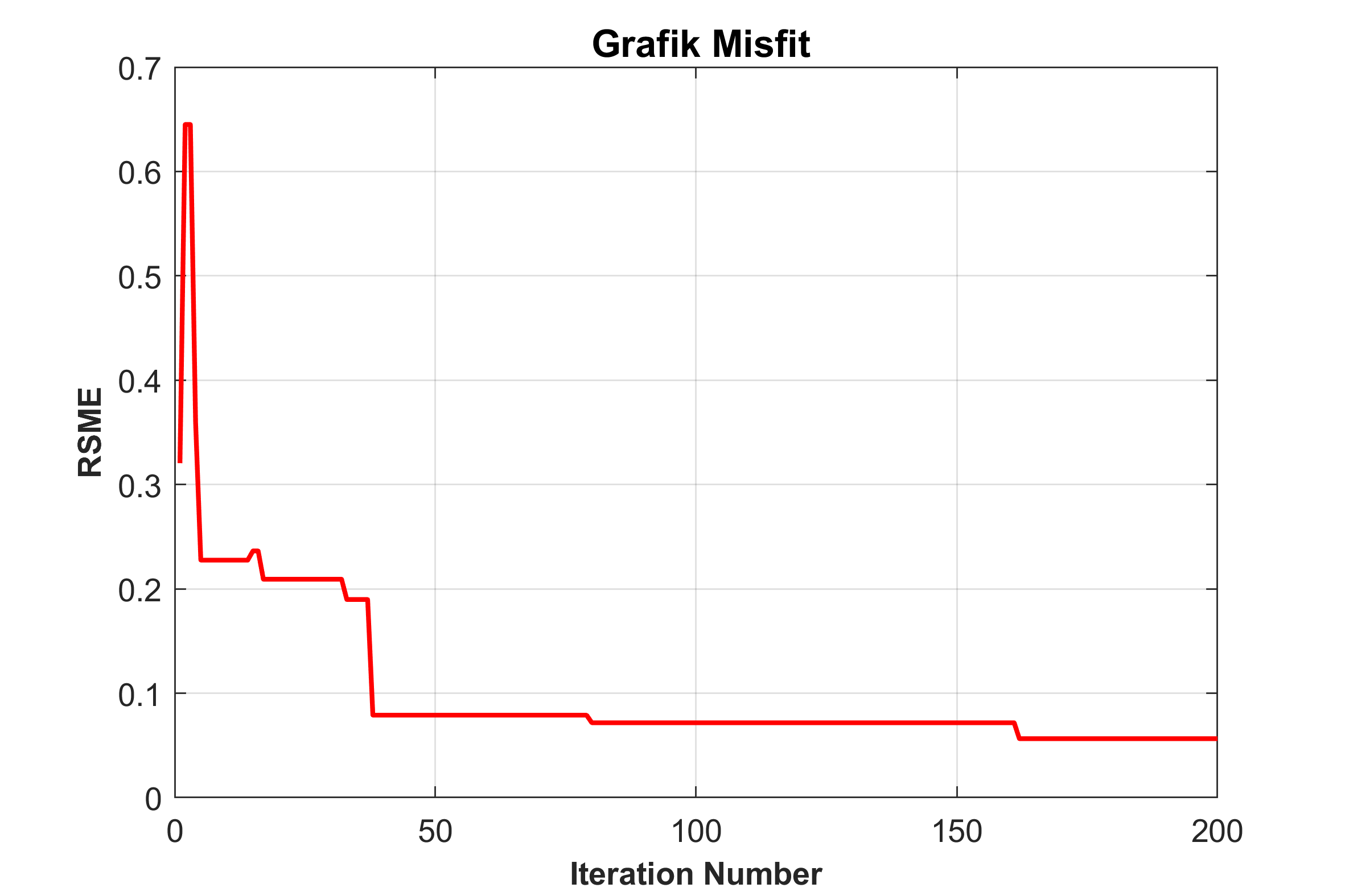
Egen(itr)=E1;
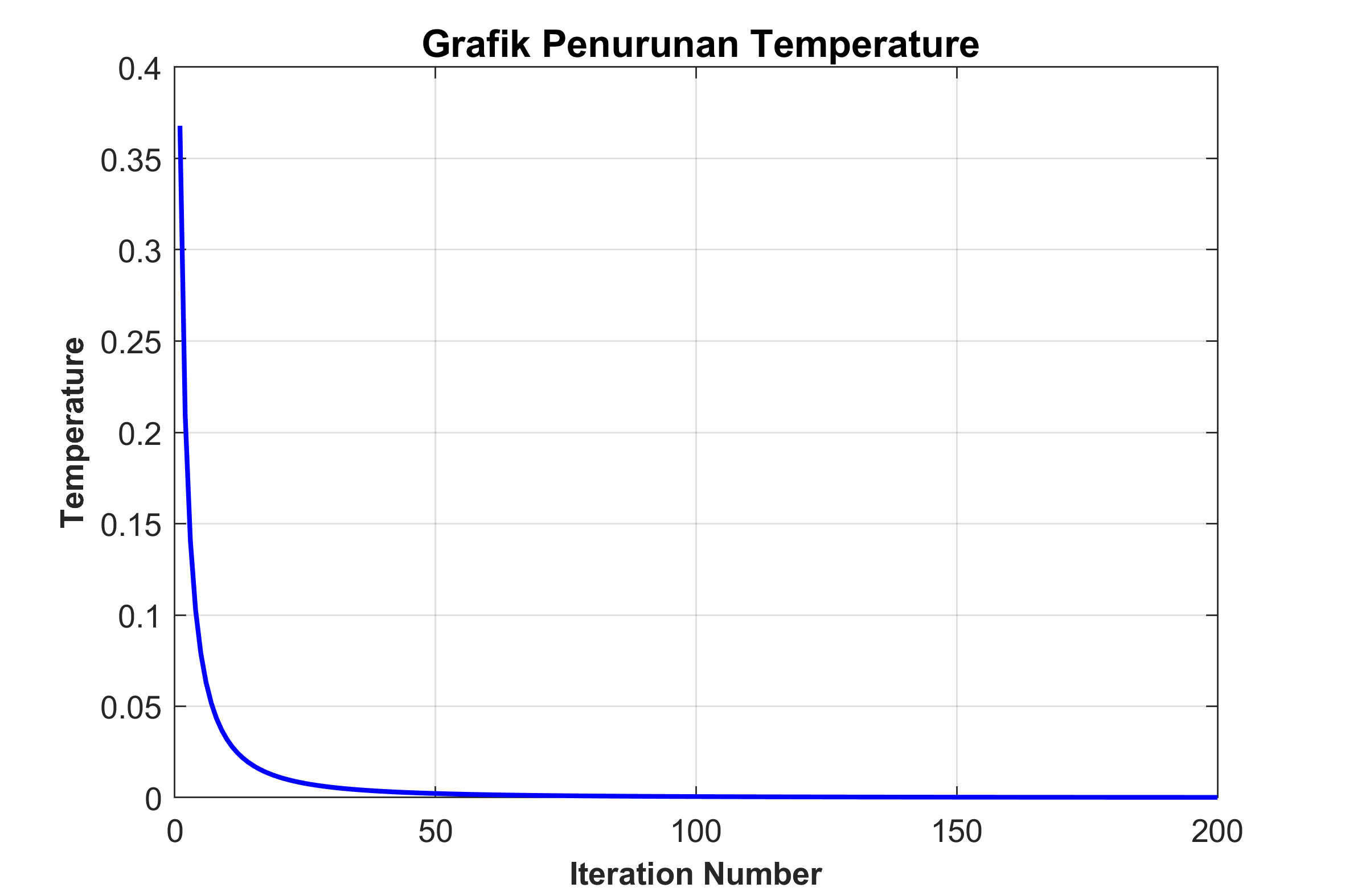
Temp = Temp*exp(-dec*(itr)^(1/(2*nlayer)-1));
Temperature(itr) = Temp;
rho_plot = [0 R];
thk_plot = [0 cumsum(thk) max(thk)*10000];
rhomod_plot = [0 rho1];
thkmod_plot = [0 cumsum(thick1) max(thick1)*10000];
end
toc
figure(1)
subplot(2, 2, 1)
loglog(T,app_sin,'.b',T,apparentResistivity_new,'r','MarkerSize',12,'LineWidth',1.5);
axis([10^-3 10^3 1 10^3]);
legend({'Synthetic Data','Calculated Data'},'EdgeColor','none','Color','none','FontWeight','Bold');
xlabel('Periods (s)','FontSize',12,'FontWeight','Bold');
ylabel('App. Resistivity (Ohm.m)','FontSize',12,'FontWeight','Bold');
title(['\bf \fontsize{10}\fontname{Times}Period (s) vs Apparent Resistivity (ohm.m) || Misfit : ', num2str(Egen(itr)),' || iteration : ', num2str(itr)]);
grid on
subplot(2, 2, 3)
loglog(T,phase_sin,'.b',T,phase_new,'r','MarkerSize',12,'LineWidth',1.5);
axis([10^-3 10^3 0 90]);
set(gca, 'YScale', 'linear');
legend({'Synthetic Data','Calculated Data'},'EdgeColor','none','Color','none','FontWeight','Bold');
xlabel('Periods (s)','FontSize',12,'FontWeight','Bold');
ylabel('Phase (deg)','FontSize',12,'FontWeight','Bold');
title(['\bf \fontsize{10}\fontname{Times}Period (s) vs Phase (deg) || Misfit : ', num2str(Egen(itr)),' || iteration : ', num2str(itr)]);
grid on
subplot(2, 2, [2 4])
stairs(rho_plot,thk_plot,'--b','Linewidth',1.5);
hold on
stairs(rhomod_plot ,thkmod_plot,'-r','Linewidth',2);
hold off
legend({'Synthetic Model','Calculated Model'},'EdgeColor','none','Color','none','FontWeight','Bold','Location','SouthEast');
axis([1 10^4 0 5000]);
xlabel('Resistivity (Ohm.m)','FontSize',12,'FontWeight','Bold');
ylabel('Depth (m)','FontSize',12,'FontWeight','Bold');
title(['\bf \fontsize{10}\fontname{Times}Model']);
subtitle(['\rho_{1} = ',num2str(rho1(1)),' || \rho_{2} = ',num2str(rho1(2)),' || \rho_{3} = ',num2str(rho1(3)),' || thick_{1} = ',num2str(thick1(1)),' || thick_{2} = ',num2str(thick1(2))],'FontWeight','bold')
set(gca,'YDir','Reverse');
set(gca, 'XScale', 'log');
set(gcf, 'Position', get(0, 'Screensize'));
grid on
figure(2)
plot(1:nitr,Egen,'r','Linewidth',1.5)
xlabel('Iteration Number','FontSize',10,'FontWeight','Bold');
ylabel('RSME','FontSize',10,'FontWeight','Bold');
title('\bf \fontsize{12} Grafik Misfit ');
set(gcf, 'Position', get(0, 'Screensize'));
grid on
figure(3)
plot(1:nitr,Temperature,'b','Linewidth',1.5)
xlabel('Iteration Number','FontSize',10,'FontWeight','Bold');
ylabel('Temperature','FontSize',10,'FontWeight','Bold');
title('\bf \fontsize{12} Grafik Penurunan Temperature ');
set(gcf, 'Position', get(0, 'Screensize'));
grid on
|