1
2
3
4
5
6
7
8
9
10
11
12
13
14
15
16
17
18
19
20
21
22
23
24
25
26
27
28
29
30
31
32
33
34
35
36
37
38
39
40
41
42
43
44
45
46
47
48
49
50
51
52
53
54
55
56
57
58
59
60
61
62
63
64
65
66
67
68
69
70
71
72
73
74
75
76
77
78
79
80
81
82
83
84
85
86
87
88
89
90
91
92
93
94
95
96
97
98
99
100
101
102
103
104
105
106
107
108
109
110
111
112
113
114
115
116
117
118
119
120
121
122
123
124
125
126
|
tic
clear all;
clc;
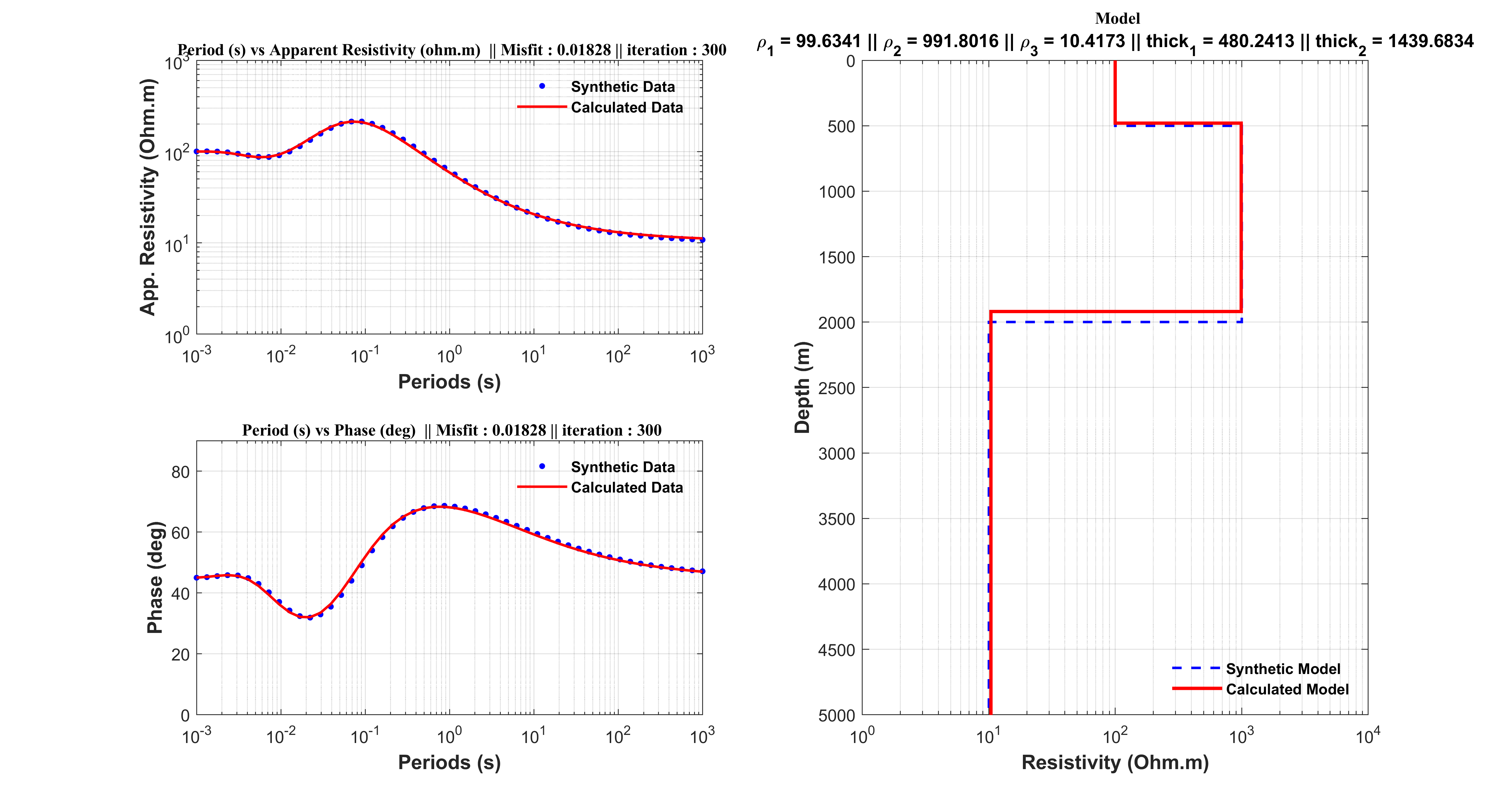
R = [100 1000 10];
thk = [500 1500];
freq = logspace(-3,3,50);
T = 1./freq;
[app_sin, phase_sin] = modelMT(R, thk ,T);
nlayer = 3;
nitr = 300;
LBR = [1 1 1];
UBR = [200 2000 20];
LBT = [1 1];
UBT = [1000 3000];
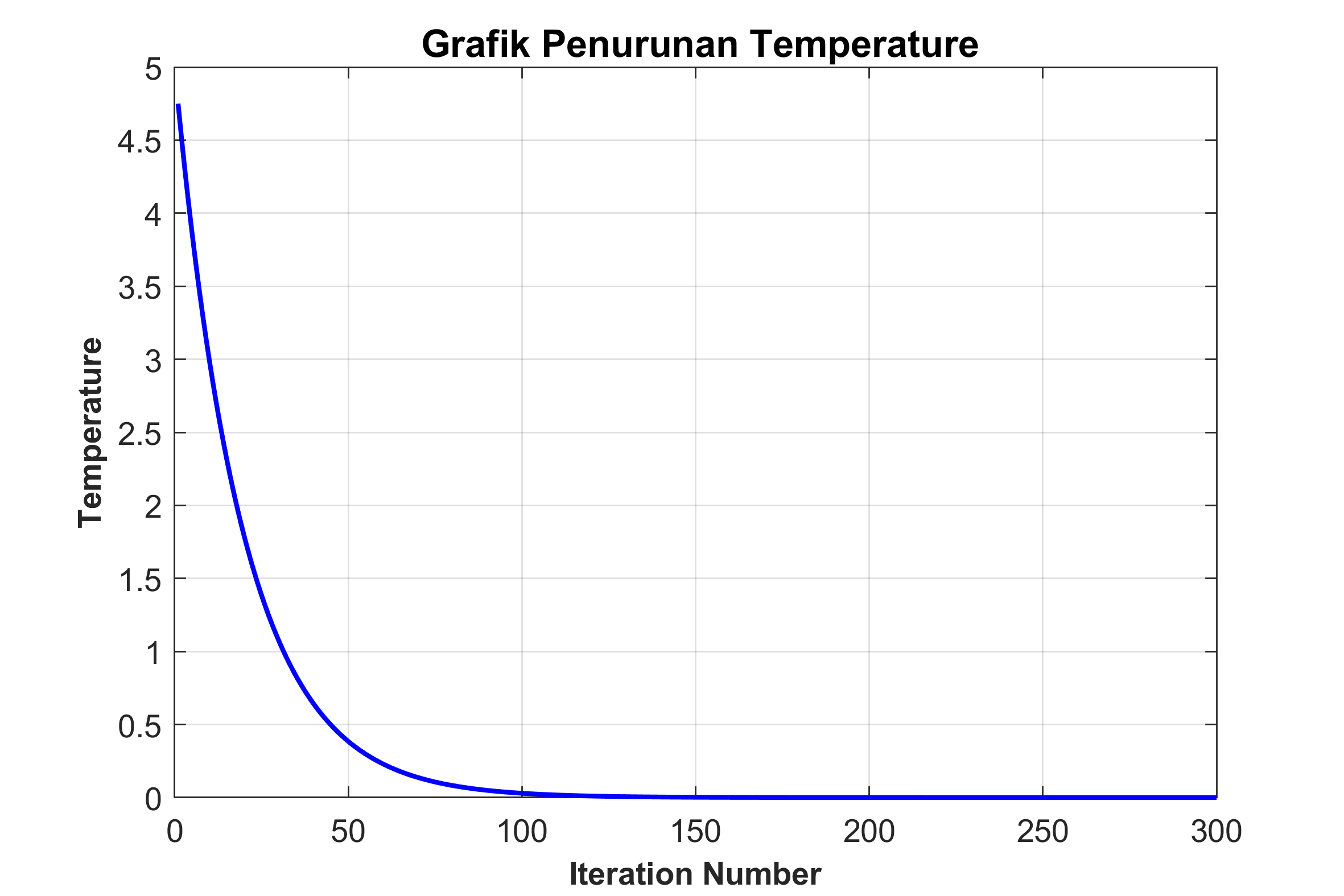
Temp = 5;
dec = 0.05;
rho1(1 , :) = LBR + rand*(UBR - LBR);
thick1(1, :) = LBT + rand*(UBT - LBT);
[apparentResistivity1, phase1]=modelMT(rho1(1,:),thick1(1,:),T);
app_mod1(1,:)=apparentResistivity1;
phase_mod1(1,:)=phase1;
[misfit1]=misfitMT(app_sin,phase_sin,app_mod1(1,:),phase_mod1(1,:));
E1=misfit1;
for itr = 1 : nitr
rho2(1 , :) = LBR + rand*(UBR - LBR);
thick2(1, :) = LBT + rand*(UBT - LBT);
[apparentResistivity2, phase2]=modelMT(rho2(1,:),thick2(1,:),T);
app_mod2(1,:)=apparentResistivity2;
phase_mod2(1,:)=phase2;
[misfit2]=misfitMT(app_sin,phase_sin,app_mod2(1,:),phase_mod2(1,:));
E2=misfit2;
delta_E = E2 -E1;
if delta_E < 0
rho1 = rho2;
thick1 = thick2;
E1 = E2;
else
P = exp((-delta_E)/Temp);
if P >= rand
rho1 = rho2;
thick1 = thick2;
E1 = E2;
end
end
[apparentResistivity_new, phase_new]=modelMT(rho1(1,:),thick1(1,:),T);
Egen(itr)=E1;
Temp = Temp*(1-dec);
Temperature(itr) = Temp;
rho_plot = [0 R];
thk_plot = [0 cumsum(thk) max(thk)*10000];
rhomod_plot = [0 rho1];
thkmod_plot = [0 cumsum(thick1) max(thick1)*10000];
end
toc
figure(1)
subplot(2, 2, 1)
loglog(T,app_sin,'.b',T,apparentResistivity_new,'r','MarkerSize',12,'LineWidth',1.5);
axis([10^-3 10^3 1 10^3]);
legend({'Synthetic Data','Calculated Data'},'EdgeColor','none','Color','none','FontWeight','Bold');
xlabel('Periods (s)','FontSize',12,'FontWeight','Bold');
ylabel('App. Resistivity (Ohm.m)','FontSize',12,'FontWeight','Bold');
title(['\bf \fontsize{10}\fontname{Times}Period (s) vs Apparent Resistivity (ohm.m) || Misfit : ', num2str(Egen(itr)),' || iteration : ', num2str(itr)]);
grid on
subplot(2, 2, 3)
loglog(T,phase_sin,'.b',T,phase_new,'r','MarkerSize',12,'LineWidth',1.5);
axis([10^-3 10^3 0 90]);
set(gca, 'YScale', 'linear');
legend({'Synthetic Data','Calculated Data'},'EdgeColor','none','Color','none','FontWeight','Bold');
xlabel('Periods (s)','FontSize',12,'FontWeight','Bold');
ylabel('Phase (deg)','FontSize',12,'FontWeight','Bold');
title(['\bf \fontsize{10}\fontname{Times}Period (s) vs Phase (deg) || Misfit : ', num2str(Egen(itr)),' || iteration : ', num2str(itr)]);
grid on
subplot(2, 2, [2 4])
stairs(rho_plot,thk_plot,'--b','Linewidth',1.5);
hold on
stairs(rhomod_plot ,thkmod_plot,'-r','Linewidth',2);
hold off
legend({'Synthetic Model','Calculated Model'},'EdgeColor','none','Color','none','FontWeight','Bold','Location','SouthEast');
axis([1 10^4 0 5000]);
xlabel('Resistivity (Ohm.m)','FontSize',12,'FontWeight','Bold');
ylabel('Depth (m)','FontSize',12,'FontWeight','Bold');
title(['\bf \fontsize{10}\fontname{Times}Model']);
subtitle(['\rho_{1} = ',num2str(rho1(1)),' || \rho_{2} = ',num2str(rho1(2)),' || \rho_{3} = ',num2str(rho1(3)),' || thick_{1} = ',num2str(thick1(1)),' || thick_{2} = ',num2str(thick1(2))],'FontWeight','bold')
set(gca,'YDir','Reverse');
set(gca, 'XScale', 'log');
set(gcf, 'Position', get(0, 'Screensize'));
grid on
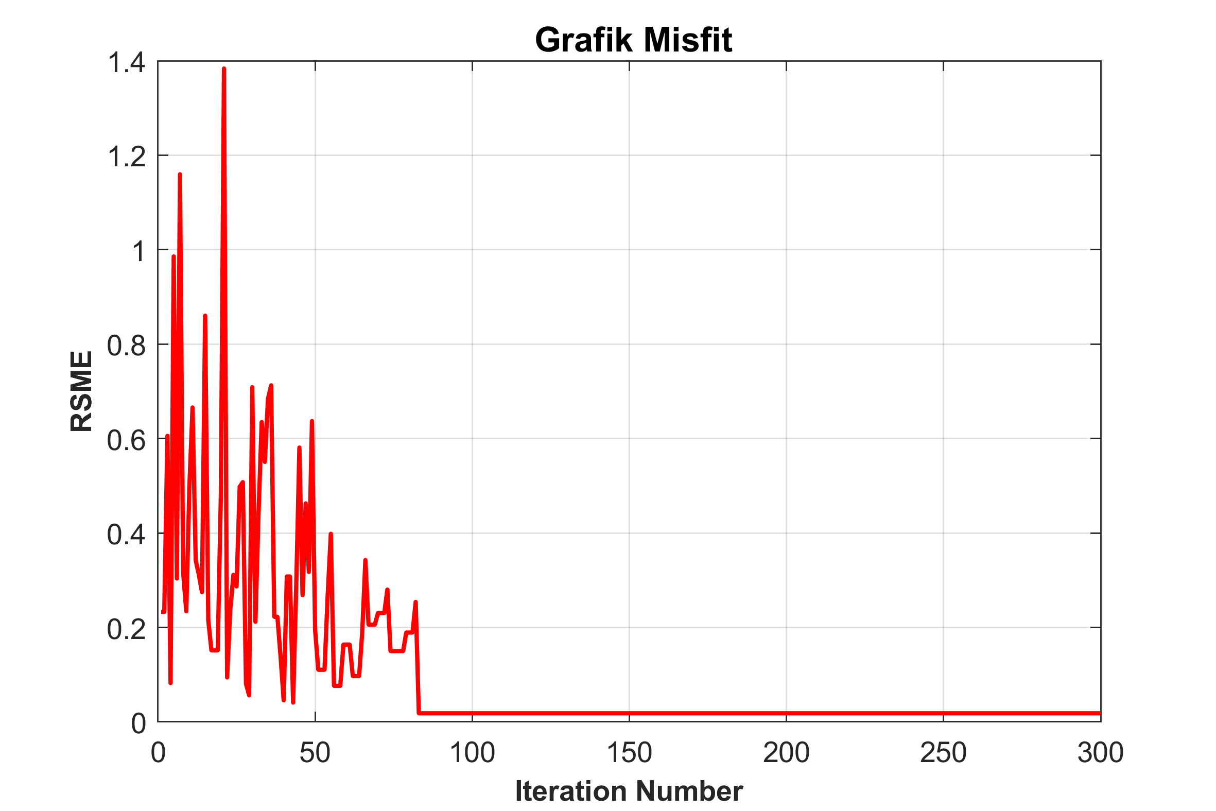
figure(2)
plot(1:nitr,Egen,'r','Linewidth',1.5)
xlabel('Iteration Number','FontSize',10,'FontWeight','Bold');
ylabel('RSME','FontSize',10,'FontWeight','Bold');
title('\bf \fontsize{12} Grafik Misfit ');
set(gcf, 'Position', get(0, 'Screensize'));
grid on
figure(3)
plot(1:nitr,Temperature,'b','Linewidth',1.5)
xlabel('Iteration Number','FontSize',10,'FontWeight','Bold');
ylabel('Temperature','FontSize',10,'FontWeight','Bold');
title('\bf \fontsize{12} Grafik Penurunan Temperature ');
set(gcf, 'Position', get(0, 'Screensize'));
grid on
|