1
2
3
4
5
6
7
8
9
10
11
12
13
14
15
16
17
18
19
20
21
22
23
24
25
26
27
28
29
30
31
32
33
34
35
36
37
38
39
40
41
42
43
44
45
46
47
48
49
50
51
52
53
54
55
56
57
58
59
60
61
62
63
64
65
66
67
68
69
70
71
72
73
74
75
76
77
78
79
80
81
82
83
84
85
86
87
88
89
90
91
92
93
94
95
96
97
98
99
100
101
102
103
104
105
106
107
108
109
110
111
112
113
114
115
116
117
118
119
120
121
122
123
124
125
126
127
128
129
130
131
132
133
134
135
136
137
138
139
140
141
142
143
144
145
146
147
148
149
150
151
152
153
154
155
156
157
158
159
160
161
162
163
|
tic
clear all;
clc;
R = [500 100 1000];
thk = [500 1500];
freq = logspace(-3,3,50);
T = 1./freq;
[app_sin, phase_sin] = modelMT(R, thk ,T);
npop = 100;
nlayer = 3;
nitr = 1000;
LBR = [1 1 1];
UBR = [2000 2000 2000];
LBT = [1 1];
UBT = [2000 2000];
wmax = 0.9;
wmin = 0.5;
c1=2.05;
c2 =2.05;
for ipop = 1 : npop
rho(ipop , :) = LBR + rand*(UBR - LBR);
thick(ipop, :) = LBT + rand*(UBT - LBT);
end
for ipop = 1 : npop
for imod = 1 : nlayer
v_rho(ipop,imod) = 0;
end
for imod = 1 : nlayer -1
v_thk(ipop,imod) = 0;
end
end
for ipop=1:npop
[apparentResistivity, phase_baru]=modelMT(rho(ipop,:),thick(ipop,:),T);
app_mod(ipop,:)=apparentResistivity;
phase_mod(ipop,:)=phase_baru;
[misfit]=misfitMT(app_sin,phase_sin,app_mod(ipop,:),phase_mod(ipop,:));
E(ipop)=misfit;
end
idx = find(E ==min(E));
G_best_rho = rho(idx(1),:);
G_best_thick = thick(idx(1),:);
for itr = 1 : nitr
w = wmax-((wmax-wmin)/nitr)*itr;
for i = 1 : npop
P_best_rho = rho;
P_best_thick = thick;
for imod = 1 : nlayer
v_rho(1,imod) = w.*v_rho(i,imod) + c1.*rand.*(P_best_rho(i,imod) - rho(i,imod))+ c2.*rand.*(G_best_rho(imod) - rho(i,imod));
rho_baru(1,imod) = rho(i,imod)+ v_rho(1,imod);
if rho_baru(1,imod)<LBR(imod)
rho_baru(1,imod) = LBR(imod);
end
if rho_baru(1,imod)>UBR(imod)
rho_baru(1,imod) = UBR(imod);
end
end
for imod = 1 : (nlayer-1)
v_thk(1,imod) = w.*v_thk(i,imod) + c1.*rand.*(P_best_thick(i,imod) - thick(i,imod))+ c2.*rand.*(G_best_thick(imod) - thick(i,imod));
thick_baru(1,imod) = thick(i,imod)+ v_thk(1,imod);
if thick_baru(1,imod)<LBT(imod)
thick_baru(1,imod) = LBT(imod);
end
if thick_baru(1,imod)>UBT(imod)
thick_baru(1,imod) = UBT(imod);
end
end
[apparentResistivity_baru, phase_baru]=modelMT(rho_baru,thick_baru,T);
app_mod_baru = apparentResistivity_baru;
phase_mod_baru(i,:) = phase_baru;
[E_baru] = misfitMT(app_sin,phase_sin,app_mod_baru, phase_mod_baru);
if E_baru<E(i)
rho(i,:) = rho_baru(1,:);
thick(i,:) = thick_baru(1,:);
app_mod(i,:) = app_mod_baru;
phase_mod(i,:) = phase_mod_baru(1,:);
E(i) = E_baru;
end
end
Emin = 100;
for ipop = 1 : npop
if E(ipop)< Emin
Emin = E(ipop);
G_best_rho = P_best_rho(ipop,:);
G_best_thick = P_best_thick(ipop,:);
app_model= app_mod(ipop,:);
phase_model = phase_mod(ipop,:);
end
end
Egen(itr)=Emin;
end
toc
rho_plot = [0 R];
thk_plot = [0 cumsum(thk) max(thk)*10000];
rhomod_plot = [0 G_best_rho];
thkmod_plot = [0 cumsum(G_best_thick ) max(G_best_thick )*10000];
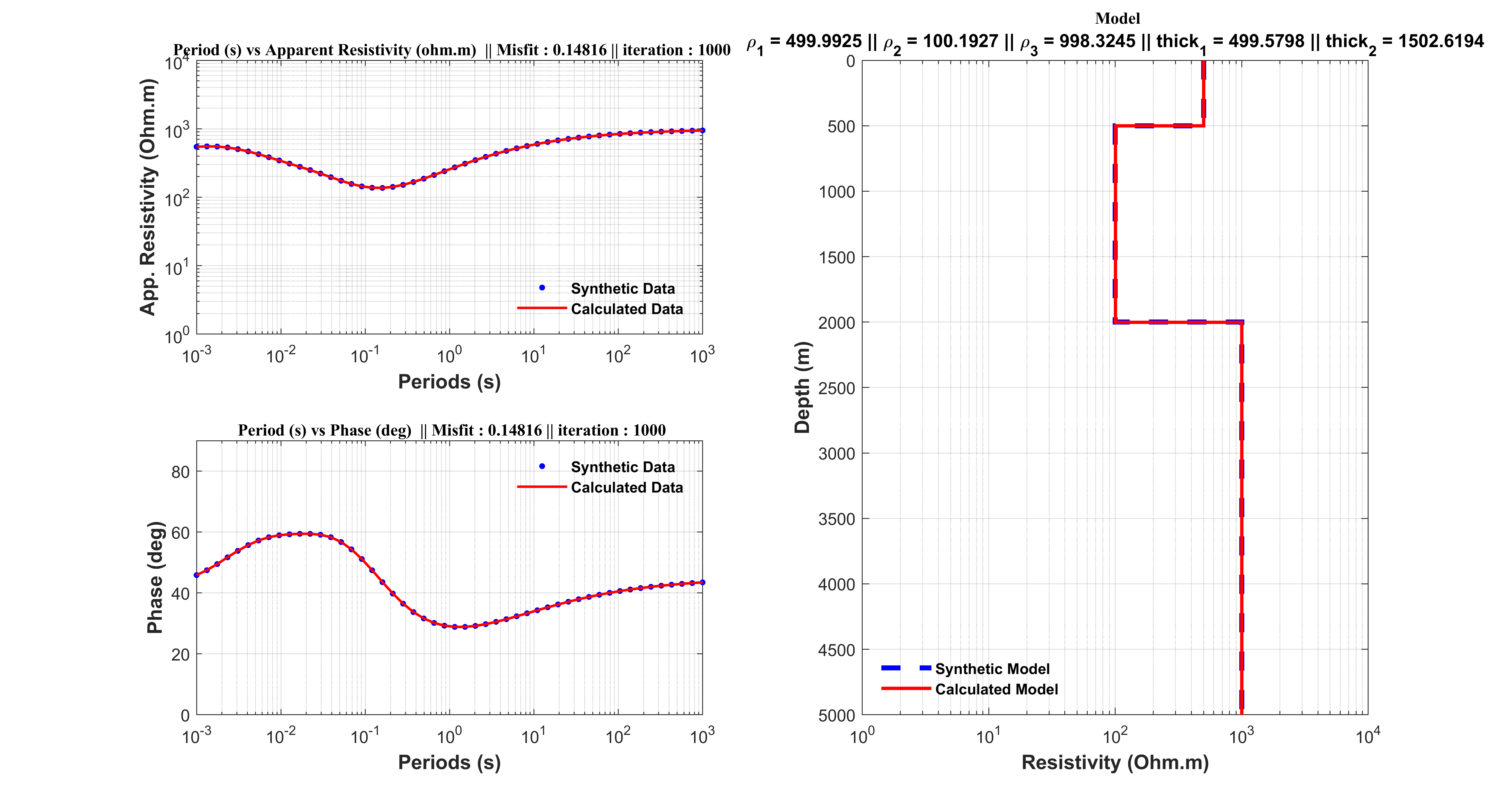
figure(1)
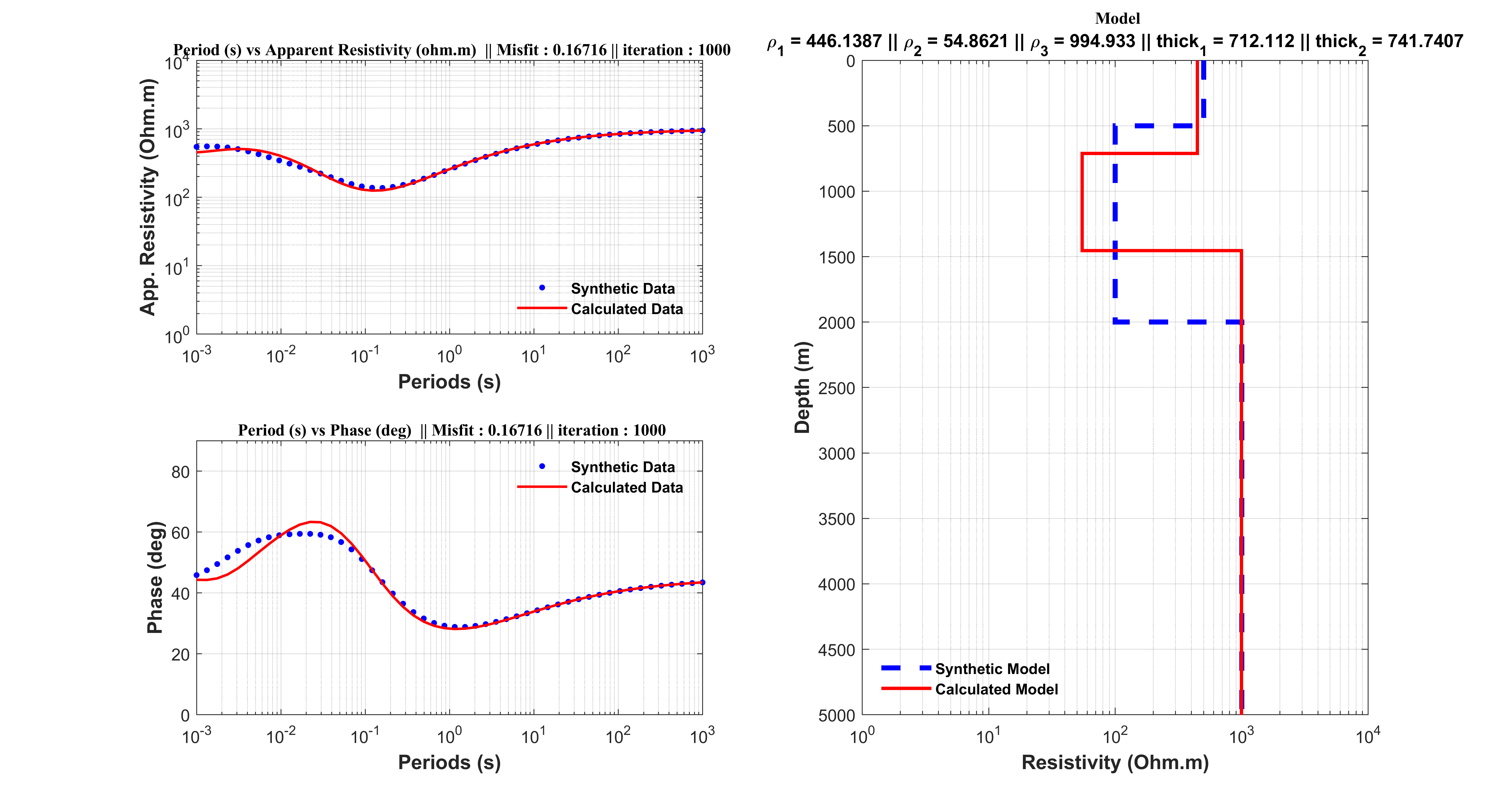
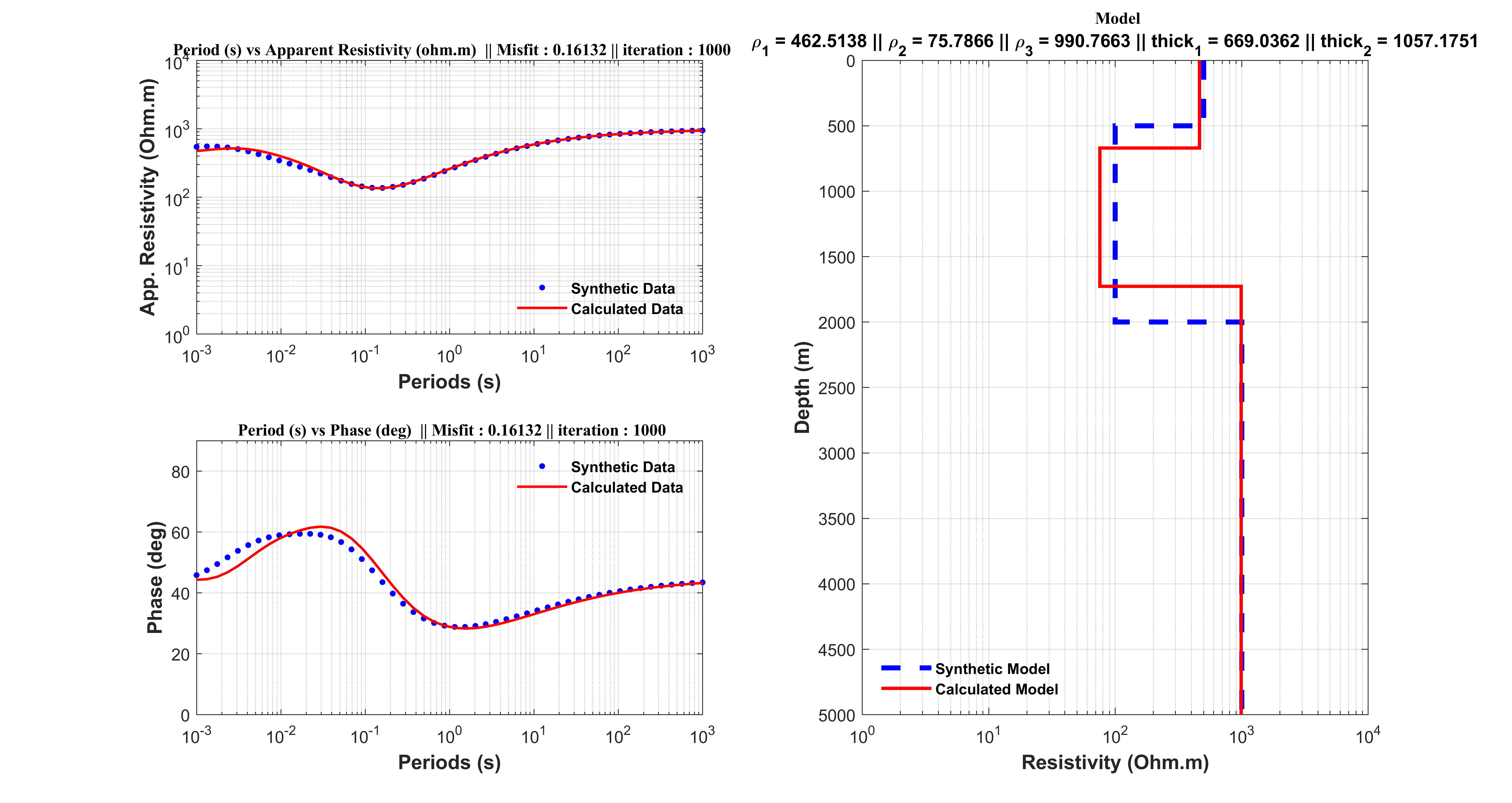
subplot(2, 2, 1)
loglog(T,app_sin,'.b',T,app_model,'r','MarkerSize',12,'LineWidth',1.5);
axis([10^-3 10^3 1 10^4]);
legend({'Synthetic Data','Calculated Data'},'EdgeColor','none','Color','none','FontWeight','Bold','location','southeast');
xlabel('Periods (s)','FontSize',12,'FontWeight','Bold');
ylabel('App. Resistivity (Ohm.m)','FontSize',12,'FontWeight','Bold');
title(['\bf \fontsize{10}\fontname{Times}Period (s) vs Apparent Resistivity (ohm.m) || Misfit : ', num2str(Egen(itr)),' || iteration : ', num2str(itr)]);
grid on
subplot(2, 2, 3)
loglog(T,phase_sin,'.b',T,phase_model,'r','MarkerSize',12,'LineWidth',1.5);
axis([10^-3 10^3 0 90]);
set(gca, 'YScale', 'linear');
legend({'Synthetic Data','Calculated Data'},'EdgeColor','none','Color','none','FontWeight','Bold');
xlabel('Periods (s)','FontSize',12,'FontWeight','Bold');
ylabel('Phase (deg)','FontSize',12,'FontWeight','Bold');
title(['\bf \fontsize{10}\fontname{Times}Period (s) vs Phase (deg) || Misfit : ', num2str(Egen(itr)),' || iteration : ', num2str(itr)]);
grid on
subplot(2, 2, [2 4])
stairs(rho_plot,thk_plot,'--b','Linewidth',3);
hold on
stairs(rhomod_plot ,thkmod_plot,'-r','Linewidth',2);
hold off
legend({'Synthetic Model','Calculated Model'},'EdgeColor','none','Color','none','FontWeight','Bold','Location','SouthWest');
axis([1 10^4 0 5000]);
xlabel('Resistivity (Ohm.m)','FontSize',12,'FontWeight','Bold');
ylabel('Depth (m)','FontSize',12,'FontWeight','Bold');
title(['\bf \fontsize{10}\fontname{Times}Model']);
subtitle(['\rho_{1} = ',num2str(G_best_rho(1)),' || \rho_{2} = ',num2str(G_best_rho(2)),' || \rho_{3} = ',num2str(G_best_rho(3)),' || thick_{1} = ',num2str(G_best_thick(1)),' || thick_{2} = ',num2str(G_best_thick(2))],'FontWeight','bold')
set(gca,'YDir','Reverse');
set(gca, 'XScale', 'log');
set(gcf, 'Position', get(0, 'Screensize'));
grid on
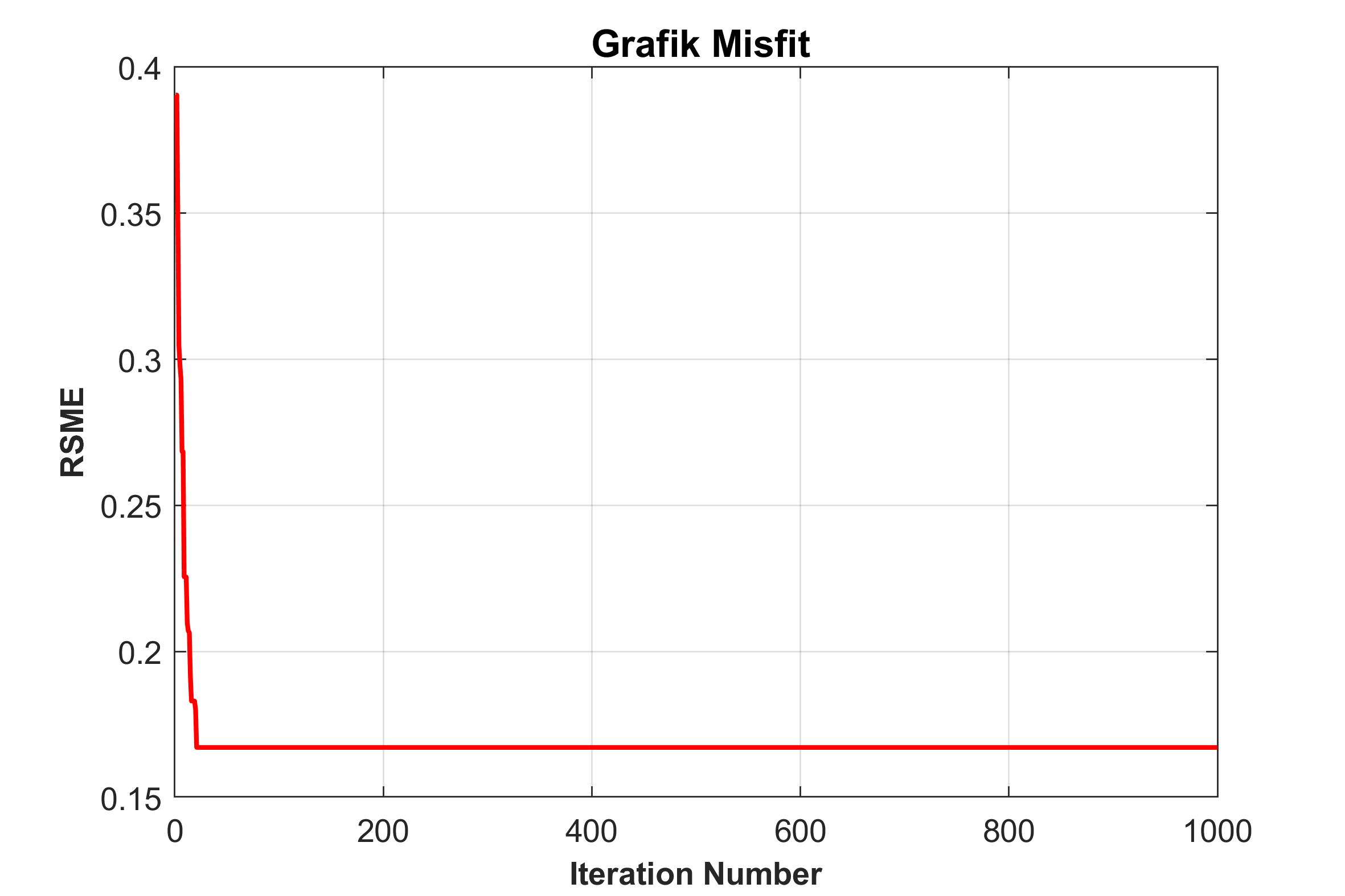
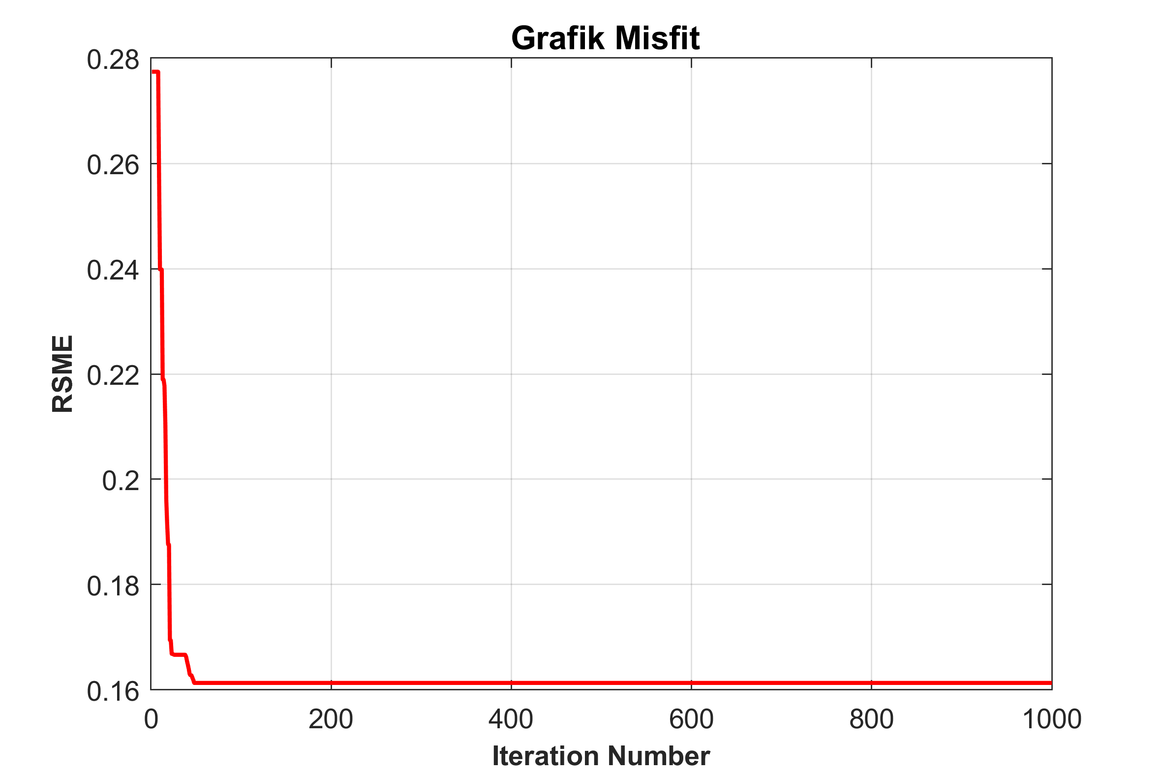
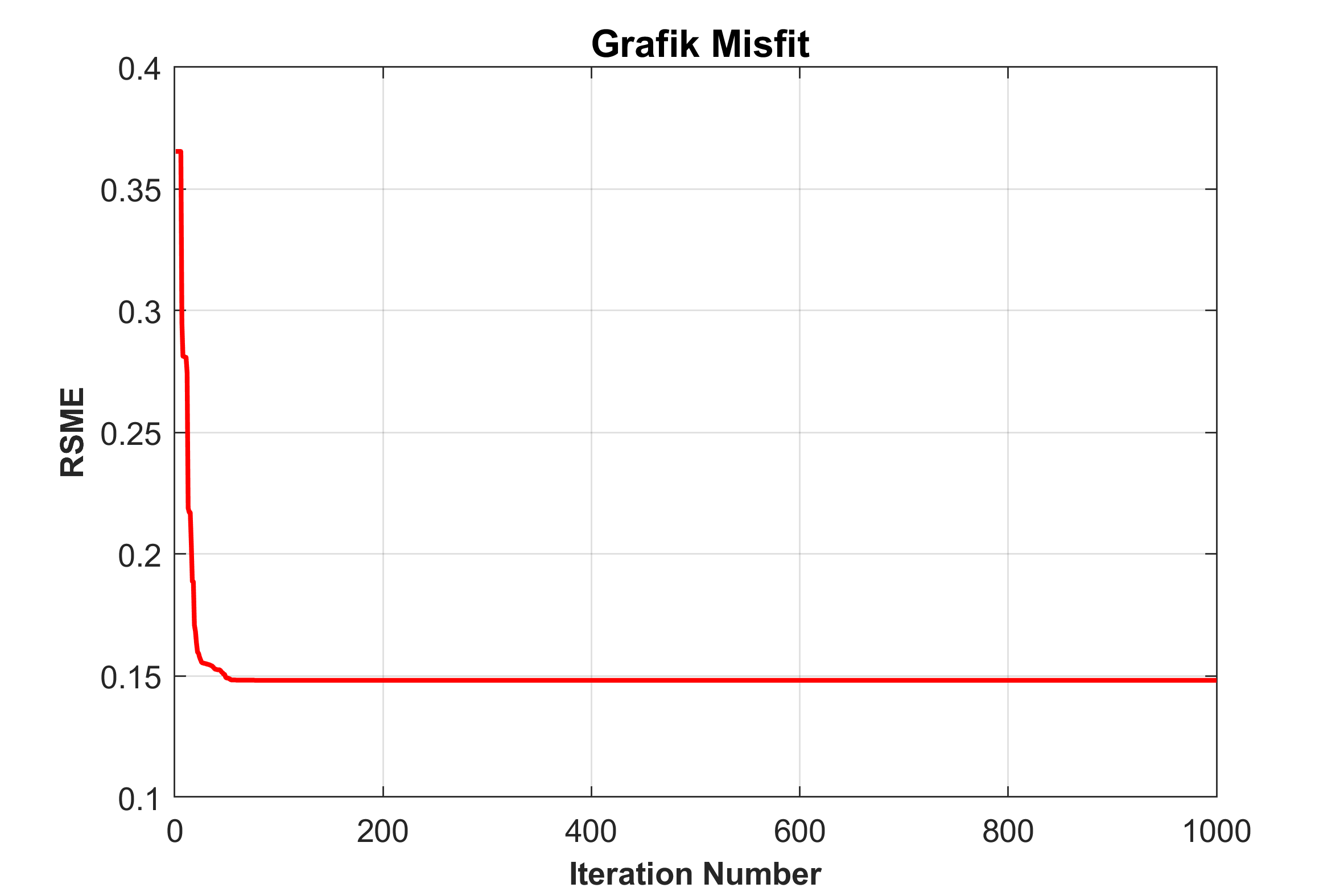
figure(2)
plot(1:nitr,Egen,'r','Linewidth',1.5)
xlabel('Iteration Number','FontSize',10,'FontWeight','Bold');
ylabel('RSME','FontSize',10,'FontWeight','Bold');
title('\bf \fontsize{12} Grafik Misfit ');
grid on
|