Bostick大地电磁一维反演 | matlab和python代码实现

Bostick是一种近似的大地电磁反演方法。这里介绍Bostick大地电磁一维反演的matlab和python程序。

Bostick反演的基本公式$^{[1]}$：

$D =\sqrt{\frac{\rho_a(T)}{\omega u_0}}=\sqrt{\frac{\rho_a(T)T}{2\pi u_0}}$ $\rho=\rho_a(T)(\frac{\pi}{2\phi(T)}-1)$

式中，$D$和$\rho$分别为反演得到的深度和真实电阻率；

$\rho_a$和$\phi$分别为视电阻率和相位，通过正演计算得到；

$\omega=2\pi f=\frac{2\pi}{T}$为角频率，$T$为周期；

$u_0$为真空磁导率，$u_0=4\pi×10^{−7}𝐻/𝑚$。

matlab代码实现：

clc
clear
%% 设置模型，并合成反演数据
mu = 4*pi*1e-7;
T=logspace(-3,4,40);
rho=[10,200,10];
depth = [1,500,2000,100000];
h = diff(depth);
[apparentRho,Phase]=MT1DForward(rho,h,1./T); %正演计算
%% Bostick反演
Depth = sqrt((apparentRho.*T)./(2*pi*mu));
rho_H = apparentRho.*(180./(2*Phase)-1);
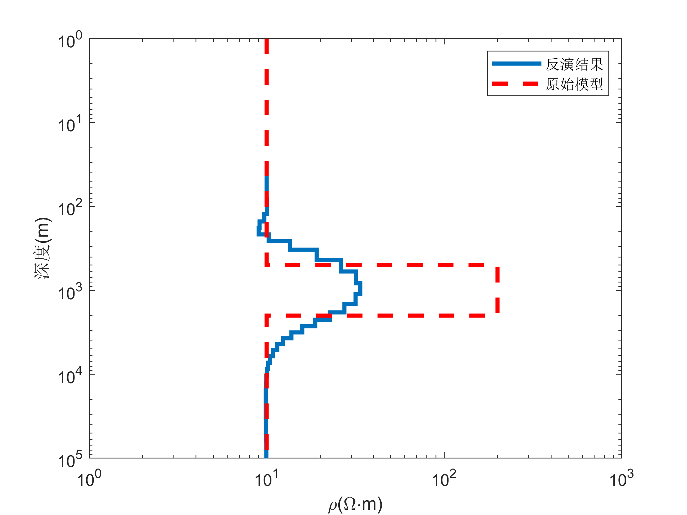
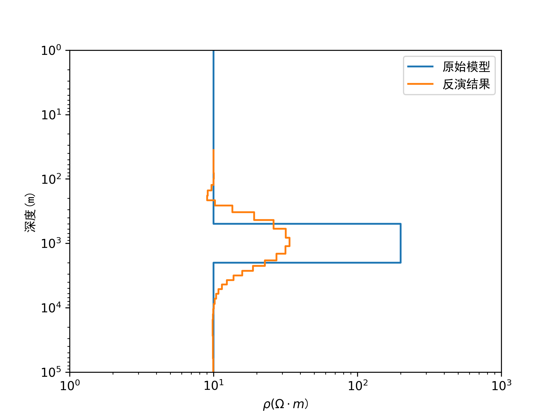
% 绘制反演结果
figure()
stairs(rho_H,Depth,'linewidth',2.5);%反演结果
hold on
rho=[10,10,200,10];
stairs(rho,depth,'r--','linewidth',2.5);%原始模型
set(gca,'xscale','log');
set(gca,'ydir','reverse','yscale','log');
xlim([1e0,1e3]);
ylim([1e0,1e5]);
xlabel('\rho(\Omega\cdotm)');
ylabel('深度(m)');
legend('反演结果','原始模型');

%% 绘制视电阻率和相位曲线对比
[apparentRho_inv,Phase_inv] = MT1DForward(rho_H,diff(Depth),1./T); 
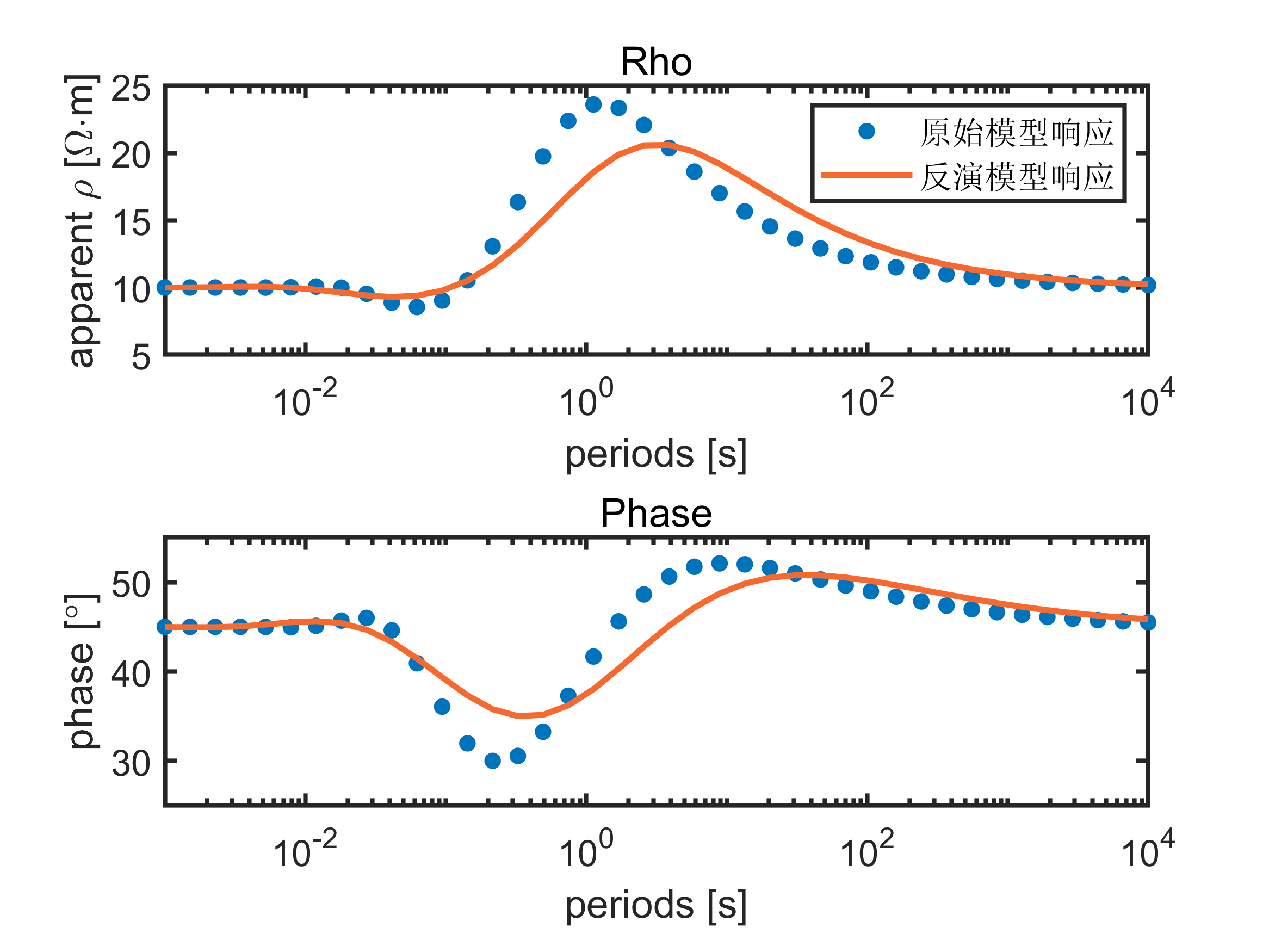
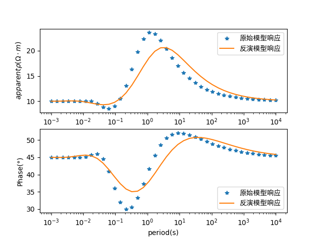
figure()
subplot(2,1,1)
    plot(T,apparentRho,'o','MarkerSize',5,'MarkerFaceColor',[0,0.45,0.74])
    hold on;
    plot(T,apparentRho_inv,'-','MarkerSize',5,'color', [0.97 0.41 0.18],'LineWidth',2)
    set(gca,'Xscale','log','LineWidth',1.5,'FontSize',12)
    xlabel('periods [s]');
    ylabel('apparent \rho [\Omega\cdotm]')
    title('Rho');
    axis([10^-3,10^4,5,25]);
    legend('原始模型响应','反演模型响应');
subplot(2,1,2)
    plot(T,Phase,'o','MarkerSize',5,'MarkerFaceColor',[0,0.45,0.74])
    hold on;
    plot(T,Phase_inv,'-','MarkerSize',5,'color', [0.97 0.41 0.18],'LineWidth',2)
    set(gca,'Xscale','log','LineWidth',1.5,'FontSize',12)
    xlabel('periods [s]');
    ylabel('phase [\circ]');
    title('Phase');
    axis([10^-3,10^4,25,55]);

其中，MT1DForward函数即“大地电磁一维正演”中提到的正演函数：

function [apparentRho,Phase] = MT1DForward(rho,h,f)  
% Notes goes here: https://cocklebur0924.github.io/2022/03/25/MT1D_Forward/
nFreqs = length(f);
nLayer = length(rho);

for iFreq = 1:nFreqs
    omega = 2*pi*f(iFreq);
    mu = 4*pi*1e-7;

for j = nLayer:-1:1
    k = sqrt(1i*omega*mu/rho(j));
    Z0 = sqrt(1i*omega*mu*rho(j));
    if j==nLayer
        Z = Z0;
        continue;
    end
    R = (Z0-Z)/(Z0+Z);
    Q = exp(-2*k*h(j));
    Z = Z0*(1-R*Q)/(1+R*Q);
end
            Z(iFreq)=Z;
            apparentRho(iFreq) = (abs(Z(iFreq)).^2)./(omega*mu);
            Phase(iFreq) = atan2d(imag(Z(iFreq)),real(Z(iFreq))); 
            % Notice:公式里计算出的相位单位为弧度，这里为°是因为使用atan2d函数转换成了度
end  
end

matlab反演结果：

反演结果

反演模型响应

python代码实现$^{[2]}$：

import numpy as np
import matplotlib.pyplot as plt
# 设置中文显示
font = {'family':'SimHei'}
plt.rcParams["axes.unicode_minus"] = False

# 定义正演函数
def MT1DForward(rho, h, T):
    mu = (4e-7)*np.pi
    nLayer = len(rho) 

    k = np.zeros((len(rho), len(T)), dtype = np.complex)
    for i in range(len(rho)):
        k[i] = np.sqrt((1j*2*np.pi*mu)/(T*rho[i]))

    Z = (2j*mu*np.pi)/(T*k[nLayer-1]) 
    layer = np.arange(nLayer-1, 0, -1) 
    for n in layer:
        A = (1j*mu*2*np.pi)/(T*k[n-1])
        B = np.exp(-2*k[n-1]*h[n-1])
        Z = A*(A*(1-B)+Z*(1+B))/(A*(1+B)+Z*(1-B))

    apparentRho = (T/(mu*2*np.pi))*(np.abs(Z)**2)
    phase = np.arctan(Z.imag/Z.real)*180/np.pi
    return [apparentRho, phase]

# 定义 bostick 反演函数
def bostick(apparentRho, phase, T):
    mu = (4e-7)*np.pi
    Depth = np.sqrt((apparentRho*T)/(2*np.pi*mu))
    rho_H = apparentRho*(180/(2*phase)-1)
    return Depth, rho_H

# 设置理论模型
T = np.logspace(-3, 4, 40)
depth = np.array([1, 500, 2000, 100000])
rho = [10, 200, 10]
h = np.diff(depth)
# 正演计算得到反演的原始数据
apparentRho, phase = MT1DForward(rho, h, T)

# 反演计算
Depth, rho_H = bostick(apparentRho, phase, T)

# 绘制反演结果图
plt.figure()
rho = [10, 10, 200, 10]
plt.plot(rho, depth, drawstyle = 'steps-post',
        label = '原始模型')
plt.plot(rho_H, Depth, drawstyle = 'steps-post',
        label = '反演结果')
# ax = plt.gca()
# ax.invert_yaxis()
plt.xlim(1e0,1e3)
plt.ylim(1e5,1e0)
plt.legend(prop = font)
plt.xlabel(r'$\rho(\Omega\cdot m$)', font)
plt.ylabel('深度(m)', font)
plt.loglog()
plt.savefig('Bostick_result_python.png', dpi =  300)

#绘制反演对比图
plt.figure()
H = np.diff(Depth)  #计算出bostick反演的层厚度
apparentRho_inv, phase_inv = MT1DForward(rho_H, H, T) # 将反演结果进行正演
# 绘制电阻率响应模型
plt.subplot(211)
plt.plot(T, apparentRho, '*', label = '原始模型响应')
plt.plot(T, apparentRho_inv, label = '反演模型响应')
plt.xlabel('period(s)')
plt.ylabel(r'$apparent \rho(\Omega\cdot m)$')
plt.semilogx()
plt.legend(prop = font)
# 绘制相位响应模型
plt.subplot(212)
plt.plot(T, phase, '*', label = '原始模型响应')
plt.plot(T, phase_inv, label = '反演模型响应')
plt.xlabel('period(s)')
plt.ylabel('Phase(°)')
plt.semilogx()
plt.legend(prop = font, loc=4)
plt.savefig('Bostick_response_python')

plt.show()