1
2
3
4
5
6
7
8
9
10
11
12
13
14
15
16
17
18
19
20
21
22
23
24
25
26
27
28
29
30
31
32
33
34
35
36
37
38
39
40
41
42
43
44
45
46
47
48
49
50
51
52
53
54
55
56
57
58
59
60
61
62
63
64
65
66
67
68
69
70
71
72
73
74
75
76
77
78
79
80
81
82
83
84
85
86
87
88
89
90
91
92
93
94
95
96
97
98
99
100
101
102
103
104
105
106
107
108
109
110
111
112
113
114
115
116
117
118
119
120
121
122
123
124
125
126
127
128
129
130
131
132
133
134
135
136
137
138
139
140
141
142
143
144
145
146
147
148
149
150
151
152
153
154
155
156
157
158
159
160
161
162
163
164
165
166
167
168
169
170
171
172
173
174
175
176
177
178
179
180
181
182
183
184
185
186
187
188
189
190
191
192
193
194
195
196
197
198
199
200
201
202
|
clc;
clear all;
R = [100 10 1000];
thk = [750 1500];
freq = logspace(-3,3,50);
nlayer = length(R);
T = 1./freq;
[app_sin, phase_sin] = modelMT(R, thk ,T);
alpha = 0.9;
gamma = 0.9;
npop = 25;
niter = 500;
fmin = 0;
fmax = 2;
for i = 1 : npop
for imod = 1 : nlayer
v_rho(i,imod) = 0;
end
for imod = 1 : nlayer -1
v_thk(i,imod) = 0;
end
end
Amin = 1;
Amax = 2;
for i = 1 : npop
for imod = 1 : nlayer
A_rho(i,imod) = Amin + rand*(Amax - Amin);
end
for imod = 1 : nlayer-1
A_thk(i,imod) = Amin + rand*(Amax - Amin);
end
end
rmin = 0;
rmax = 1;
for i = 1 : npop
for imod = 1 : nlayer
r_rho(i,imod) = rmin + rand*(rmax-rmin);
end
for imod = 1 : nlayer-1
r_thk(i,imod) = rmin + rand*(rmax-rmin);
end
end
rhomin = [1 1 1];
rhomax = [2000 2000 2000];
thkmin = [1 1];
thkmax = [2000 2000];
for i = 1 : npop
rho(i , :) = rhomin + rand*(rhomax - rhomin);
thick(i, :) = thkmin + rand*(thkmax - thkmin);
end
for ipop=1:npop
[apparentResistivity, phase]=modelMT(rho(ipop,:),thick(ipop,:),T);
app_mod(ipop,:)=apparentResistivity;
phase_mod(ipop,:)=phase;
[misfit]=misfitMT(app_sin,phase_sin,app_mod(ipop,:),phase_mod(ipop,:));
E(ipop)=misfit;
end
idx = find(E ==min(E));
G_best_rho = rho(idx(1),:);
G_best_thick = thick(idx(1),:);
for itr = 1 : niter
for i = 1 : npop
for imod = 1 : nlayer
f_rho(imod) = fmin + rand*(fmin-fmax);
end
for imod = 1 : nlayer-1
f_thk(imod) = fmin + rand*(fmin-fmax);
end
for imod = 1 : nlayer
v_rho(1,imod) = v_rho(i,imod) + (rho(i,imod)-G_best_rho(imod))*f_rho(imod);
rho_baru(1,imod) = rho(i,imod) + v_rho(1,imod);
if rho_baru(1,imod) > rhomax(imod)
rho_baru(1,imod) = rhomax(imod);
end
if rho_baru(1,imod) < rhomin(imod)
rho_baru(1,imod) = rhomin(imod);
end
end
for imod = 1 : nlayer-1
v_thk(1,imod) = v_thk(i,imod) + (thick(i,imod)-G_best_thick(imod))*f_thk(imod);
thick_baru(1,imod) = thick(i,imod) +v_thk(1,imod);
if thick_baru(1,imod) > thkmax(imod)
thick_baru(1,imod) = thkmax(imod);
end
if thick_baru(1,imod) < thkmin(imod)
thick_baru(1,imod) = thkmin(imod);
end
end
random = rand;
if random > r_rho(i)
for imod = 1 : nlayer
rho_baru(1,imod) =G_best_rho(imod)+mean(A_rho(i,:))*(-1+2*rand);
end
if rho_baru(1,imod) > rhomax(imod)
rho_baru(1,imod) = rhomax(imod);
end
if rho_baru(1,imod) < rhomin(imod)
rho_baru(1,imod) = rhomin(imod);
end
end
if random > r_thk(i)
for imod = 1 : nlayer-1
thick_baru(1,imod) = G_best_thick(imod) + mean(A_thk(i,:))*(-1+2*rand);
end
if thick_baru(1,imod) > thkmax(imod)
thick_baru(1,imod) = thkmax(imod);
end
if thick_baru(1,imod) < thkmin(imod)
thick_baru(1,imod) = thkmin(imod);
end
end
[apparentResistivity_baru, phase_baru]=modelMT(rho_baru,thick_baru,T);
[E_baru] = misfitMT(app_sin,phase_sin,apparentResistivity_baru, phase_baru);
if E_baru < E(i) && rand < A_rho(i) && rand < A_thk(i)
rho(i,:) = rho_baru(1,:);
thick(i,:) = thick_baru(1,:);
E(i) = E_baru;
app_mod(i,:) = apparentResistivity_baru(1,:);
phase_mod(i,:) = phase_baru(1,:);
end
end
Emin = 1000;
for i = 1 : npop
if E(i)< Emin
Emin = E(i);
G_best_rho = rho(i,:);
G_best_thick = thick(i,:);
app_model = app_mod(i,:);
phase_model = phase_mod(i,:);
end
end
A_rho(i) = A_rho(i)*alpha;
A_thk(i) = A_thk(i)*alpha;
r_rho(i) = r_rho(i)*(1-exp(gamma*itr));
r_thk(i) = r_thk(i)*(1-exp(gamma*itr));
Egen(itr)=Emin;
rho_plot = [0 R];
thk_plot = [0 cumsum(thk) max(thk)*10000];
rhomod_plot = [0 G_best_rho];
thkmod_plot = [0 cumsum(G_best_thick) max(G_best_thick)*10000];
end
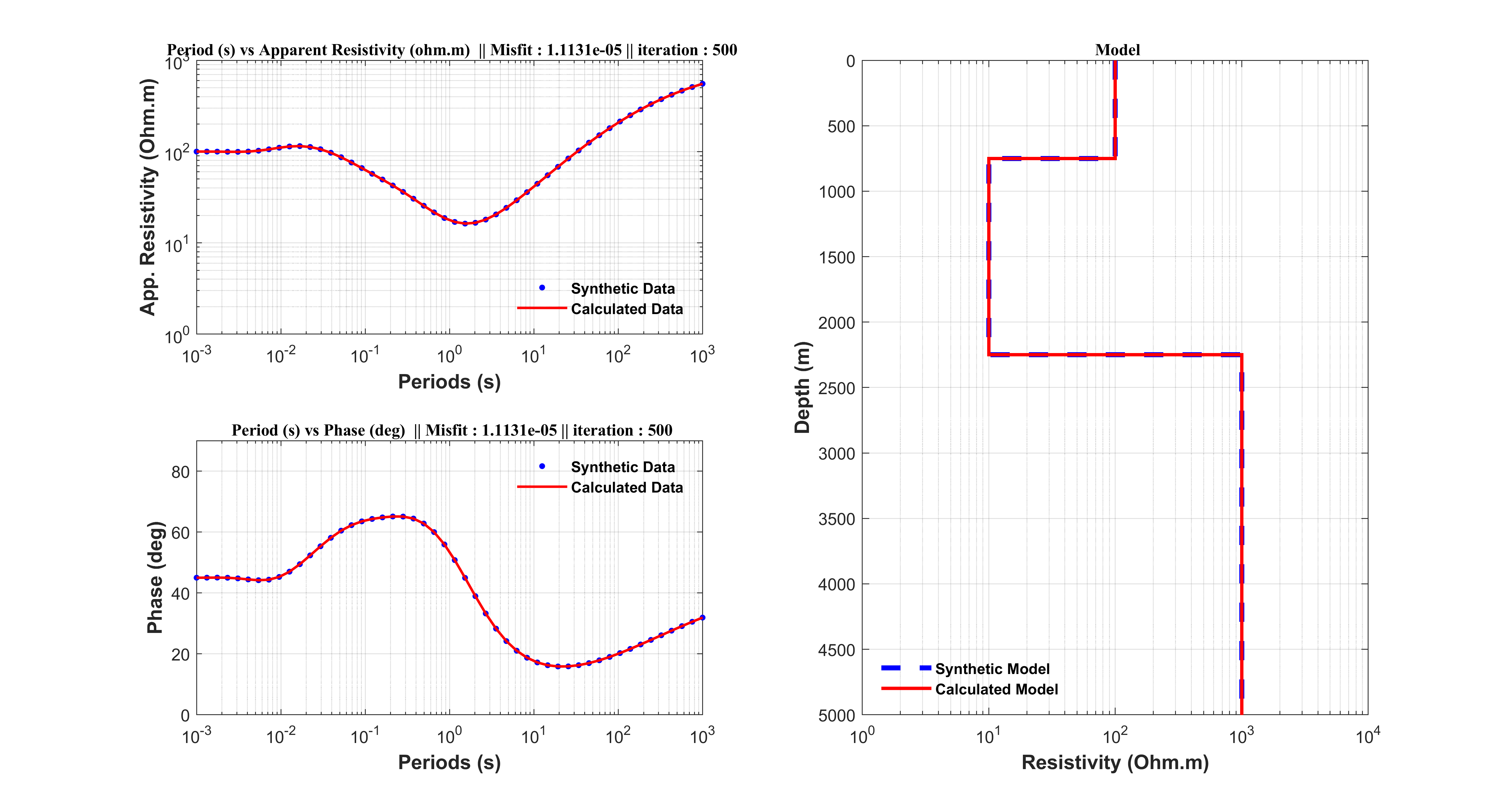
figure(1)
subplot(2, 2, 1)
loglog(T,app_sin,'.b',T,app_model,'r','MarkerSize',12,'LineWidth',1.5);
axis([10^-3 10^3 1 10^3]);
legend({'Synthetic Data','Calculated Data'},'EdgeColor','none','Color','none','FontWeight','Bold','location','SouthEast');
xlabel('Periods (s)','FontSize',12,'FontWeight','Bold');
ylabel('App. Resistivity (Ohm.m)','FontSize',12,'FontWeight','Bold');
title(['\bf \fontsize{10}\fontname{Times}Period (s) vs Apparent Resistivity (ohm.m) || Misfit : ', num2str(Egen(itr)),' || iteration : ', num2str(itr)]);
grid on
subplot(2, 2, 3)
loglog(T,phase_sin,'.b',T,phase_model,'r','MarkerSize',12,'LineWidth',1.5);
axis([10^-3 10^3 0 90]);
set(gca, 'YScale', 'linear');
legend({'Synthetic Data','Calculated Data'},'EdgeColor','none','Color','none','FontWeight','Bold');
xlabel('Periods (s)','FontSize',12,'FontWeight','Bold');
ylabel('Phase (deg)','FontSize',12,'FontWeight','Bold');
title(['\bf \fontsize{10}\fontname{Times}Period (s) vs Phase (deg) || Misfit : ', num2str(Egen(itr)),' || iteration : ', num2str(itr)]);
grid on
subplot(2, 2, [2 4])
stairs(rho_plot,thk_plot,'--b','Linewidth',3);
hold on
stairs(rhomod_plot ,thkmod_plot,'-r','Linewidth',2);
hold off
legend({'Synthetic Model','Calculated Model'},'EdgeColor','none','Color','none','FontWeight','Bold','Location','SouthWest');
axis([1 10^4 0 5000]);
xlabel('Resistivity (Ohm.m)','FontSize',12,'FontWeight','Bold');
ylabel('Depth (m)','FontSize',12,'FontWeight','Bold');
title(['\bf \fontsize{10}\fontname{Times}Model']);
set(gca,'YDir','Reverse');
set(gca, 'XScale', 'log');
set(gcf, 'Position', get(0, 'Screensize'));
grid on
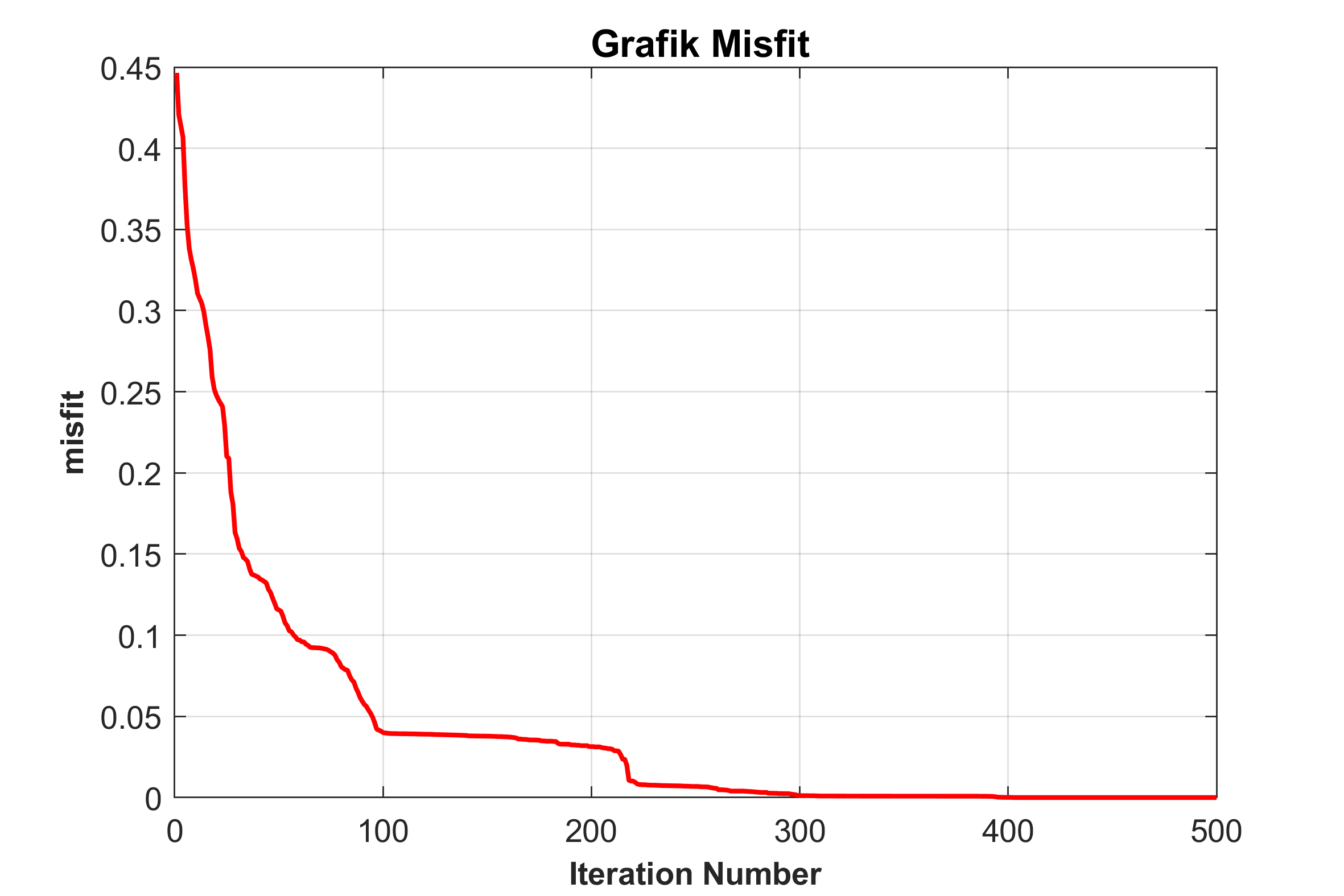
figure(2)
plot(1:niter,Egen,'r','Linewidth',1.5)
xlabel('Iteration Number','FontSize',10,'FontWeight','Bold');
ylabel('misfit','FontSize',10,'FontWeight','Bold');
title('\bf \fontsize{12} Grafik Misfit ');
grid on
|